Understanding AUROC: A Mathematical and Practical Perspective

May 3, 2025

Dive into the AUROC metric—its mathematical foundation, interpretation, and practical pros and cons in evaluating binary classification models.

In this blog, we’ll explore the AUC-ROC (Area Under the Receiver Operating Characteristic Curve), a widely used metric for evaluating the performance of binary classification models. We'll break down its interpretation, how it's calculated, and its strengths and weaknesses.

1. Confusion Matrix Basics

To understand AUC-ROC, we begin with the confusion matrix, which summarizes classification results using four components:

True Positive (TP): Positive samples correctly predicted as positive.
True Negative (TN): Negative samples correctly predicted as negative.
False Positive (FP): Negative samples incorrectly predicted as positive.
False Negative (FN): Positive samples incorrectly predicted as negative.

Confusion Matrix

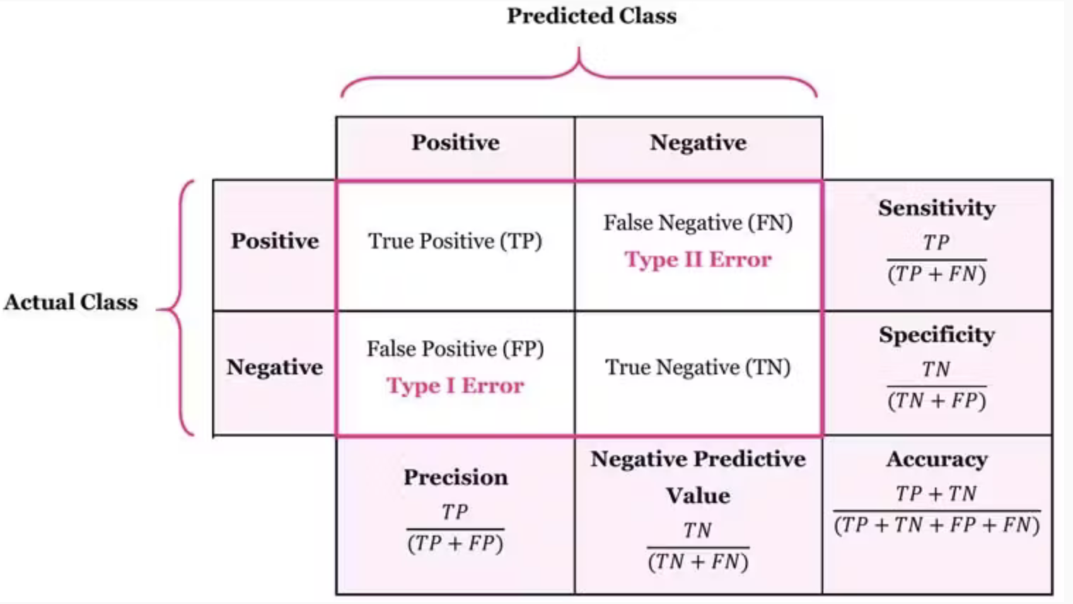
These form the basis for computing performance metrics used in ROC analysis.

2. Key Performance Metrics

Two core metrics derived from the confusion matrix are:

True Positive Rate (TPR) or Recall:
$TPR = \frac{T P}{T P + F N}$
False Positive Rate (FPR):
$FPR = \frac{F P}{F P + T N}$

These values vary depending on the classification threshold used.

3. ROC Curve and AUC

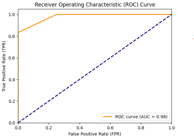
The ROC curve plots TPR (y-axis) against FPR (x-axis) at various threshold levels. Each point on the curve corresponds to a different decision threshold. The Area Under the ROC Curve (AUC) provides a single scalar value to summarize model performance:

AUC = 0.5: The model is no better than random guessing.
0.5 < AUC < 0.7: Poor performance.
0.7 ≤ AUC < 0.9: Good performance.
AUC ≥ 0.9: Excellent discrimination capability.

ROC Curve Illustration

4. Mathematical Foundation of AUROC

Let:

$X_{p}$ : A random variable representing the predicted score for a positive sample.
$X_{n}$ : A random variable representing the predicted score for a negative sample.

The TPR and FPR depend on a classification threshold $t$ , and the AUC can be mathematically defined as:

AUC = \int_{0}^{1} TPR (t) d (FPR (t))

Using cumulative distribution functions $F (.)$ , we can express:

$TPR (t) = P (X_{p} > t) = 1 - F_{X_{p}} (t)$
$FPR (t) = P (X_{n} > t) = 1 - F_{X_{n}} (t)$

Substituting into the AUC definition and simplifying, we obtain:

AUC = \int_{0}^{1} TPR (t) d (FPR (t)) = \int_{0}^{1} (1 - F_{X_{p}} (t)) d (1 - F_{X_{n}} (t)) = \int_{- \infty}^{\infty} (1 - F_{X_{p}} (t)) f_{X_{n}} (t) d t = 1 - \int_{- \infty}^{\infty} F_{X_{p}} (t) f_{X_{n}} (t) d t = 1 - E_{X_{n} \sim N} [F_{X_{p}} (X_{n})] = 1 - E_{X_{n} \sim N} [P (X_{p} < X_{n})] = P (X_{p} > X_{n})

This derivation shows that AUC represents the probability that a randomly chosen positive sample has a higher score than a randomly chosen negative sample. Therefore:

If the model always ranks positive samples above negative ones, AUC = 1.
If the model ranks randomly, AUC = 0.5.

5. Strengths and Weaknesses of AUC-ROC

✅ Advantages

Threshold-independent: AUC evaluates model performance across all possible classification thresholds, unlike accuracy which is sensitive to the chosen threshold.
Robust to class imbalance: AUC remains informative even when classes are imbalanced, unlike metrics like accuracy that can be misleading in such scenarios.

❌ Disadvantages

Does not reflect misclassification costs: AUC does not consider the varying consequences of false positives vs. false negatives, which can be critical in domains like healthcare or finance.
Interpretability can be tricky: Especially with complex models, interpreting what a specific AUC value implies in practice may not always be straightforward.

By understanding both the mathematical underpinning and practical implications of AUC-ROC, we can better evaluate binary classifiers and make informed choices in model selection and deployment.