
The Bradley–Terry–Luce Model: Turning Head-to-Head Wins into Scores
November 3, 2026 · 10 min read · Statistics, Machine Learning, Large Language Models
Contents · 8 sections
- 1. The model
- Luce's choice axiom and rankings
- 2. Fitting the scores
- The likelihood
- When does the fit exist?
- Zermelo's iteration, by hand
- How sure are we?
- 3. Experiment: how many comparisons do you need?
- 4. Where you've already met it
- Elo is BT, fitted one game at a time
- Chatbot leaderboards
- Reward models for RLHF
- 5. Common extensions
- 6. Where it breaks
- 7. In code
- Recap
Suppose you want to rank ten dishes at a food festival. There's no exam that every dish sits. All you have are judges who taste two dishes at a time and say which one they prefer. Some pairs get compared often, some once, some never. How do you turn that pile of little "A beat B" verdicts into one score per dish?
The same question shows up everywhere: chess players who only ever meet a few opponents, sports teams, search results compared side by side, and, most recently, chatbots that people vote between. The standard answer is a one-line model from the 1950s: the Bradley–Terry–Luce (BTL) model. This post covers:
- the model and the picture behind it,
- how to fit it, and when the fit doesn't exist,
- a simulation of how many comparisons you need,
- how it connects to Elo, chatbot leaderboards and RLHF,
- where it breaks.
1. The model#
Give every item a hidden positive strength . The Bradley–Terry model (Bradley and Terry, 1952; Zermelo proposed the same model for chess in 1929) says:
Here is the strength of item . If and , item wins 3 out of 4 times. Equal strengths give a coin flip.
It's easier to work with scores on the log scale, . Dividing top and bottom by gives
where is the logistic (sigmoid) function. So BT is just logistic regression on score differences:
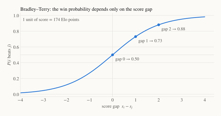
Two things follow from this picture:
- Only the gap matters. A gap of 1 means a 73% chance of winning, and a gap of 2 means 88%, whether the two players are beginners or champions.
- Scores have no absolute zero. Adding the same constant to every changes no probability. We'll have to pin the scale down when fitting.
Luce's choice axiom and rankings#
Luce (1959) generalised the idea from pairs to choosing one item out of a set :
This is Luce's choice axiom. A consequence is that the odds between and , , don't depend on what else is on the menu. Economists call this independence of irrelevant alternatives, and it will come back in the "where it breaks" section.
Applying the rule repeatedly gives a model for full rankings, the Plackett–Luce model (Plackett, 1975): pick the winner from all items, then the runner-up from the rest, and so on, multiplying the probabilities. For two items it reduces to Bradley–Terry.
2. Fitting the scores#
The likelihood#
Let be the number of games between and , and the number that won, so . Assuming games are independent, the log-likelihood of the scores is
with the number of items. This is the logistic-regression log-likelihood, so it's concave and has no local maxima to get stuck in. Its gradient has a lovely reading:
where is the total number of wins of item . The sum is the number of wins the model expects for . At the maximum the gradient is zero, so every player's expected wins equal their actual wins.
Because only gaps matter, we fix the scale by a convention: either set one reference item to (), or make the scores average to zero.
When does the fit exist?#
Ask yourself: how strong is a player who has never lost? The data only says "stronger than everyone they played". The likelihood keeps improving as their score goes up, forever. The maximum likelihood estimate (MLE) is .
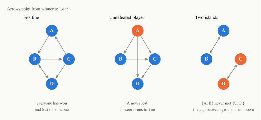
Ford (1957) gave the exact condition. Draw an arrow from each winner to each loser. A finite MLE exists if and only if, however you split the items into two groups, someone in each group has beaten someone in the other. Two common ways to fail:
- An undefeated (or winless) item: its score runs off to .
- Islands: if never played , the data can't tell how far apart the groups are.
The practical fix is a weak prior: subtract a penalty from the log-likelihood (a Gaussian prior on the scores). With a small , the estimates barely move when the data is rich, and stay finite when it isn't.
Zermelo's iteration, by hand#
Setting the gradient to zero in terms of strengths gives . Solve for while holding the denominators fixed, and you get a simple update first proposed by Zermelo:
Hunter (2004) showed this is an MM algorithm (minorise–maximise): each step is guaranteed to increase the likelihood.
Let's run it on three players who each play 3 games against each other:
| Pair | Result | Wins so far |
|---|---|---|
| A vs B | A wins 2–1 | |
| B vs C | B wins 2–1 | |
| A vs C | A wins 2–1 |
Start with . Every denominator is , so one step gives
One step already ranks the players. Repeating until nothing changes (keeping as the reference) gives
Now the interesting part: the model says , even though A beat C in only 2 of 3 games (0.667). The model borrows strength from the other games: A beat B, and B beat C, so A should be clearly better than C. That pooling is the whole point of fitting one model to all the comparisons.
How sure are we?#
Two standard ways to put error bars on the scores:
- Fisher information. The curvature of the log-likelihood is , where and is the -th unit vector. After fixing a reference item, its inverse approximates the covariance of the estimates. Close matches () are the most informative games.
- Bootstrap. Resample the games with replacement, refit, and look at the spread. It's simple and doesn't rely on large-sample formulas.
3. Experiment: how many comparisons do you need?#
Let's check on data where we know the answer. Take 10 items with true scores evenly spaced from to (so the best item beats the worst 95% of the time). Generate random pairs, decide each winner by flipping a coin with probability , fit BT with a weak prior (), and compare the estimates with the truth. For comparison we also run Elo (Section 4) once through the same games. Each dataset size is repeated 200 times; lines are medians and bands cover the middle 80%.
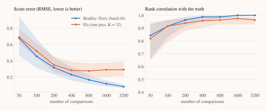
- The BT error keeps shrinking: median RMSE goes from 0.68 with 50 comparisons to 0.23 with 400 and 0.08 with 3,200. Quadrupling the data roughly halves the error, the familiar rate.
- The ranking settles early: by 400 comparisons (about 9 per pair) the median rank correlation with the truth is 0.99.
- Elo stalls: its error stops improving around 0.28–0.29 from 400 games on. With a fixed step size , every new game keeps nudging the ratings, so they never stop jittering around the truth.
Elo has a second problem: its answer depends on the order of the games. Here is one dataset of 400 games. BT gives a single estimate per item (with a bootstrap interval for sampling uncertainty). Elo's ratings change just by shuffling the same games:
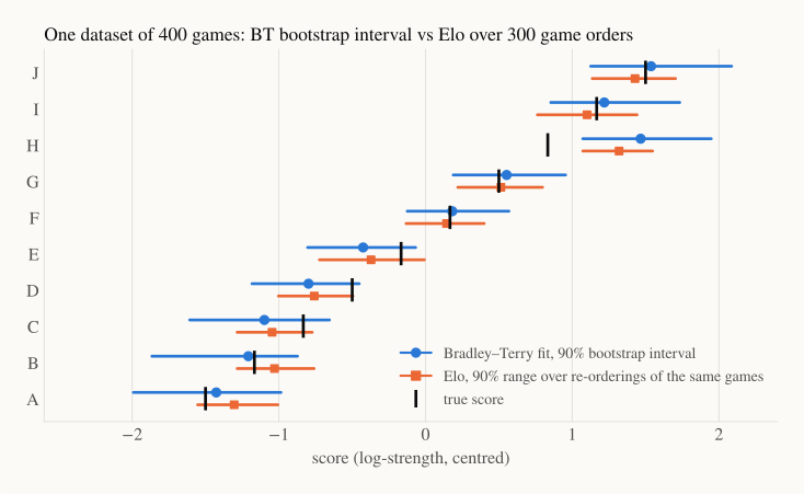
With the data held fixed, reordering alone moves Elo scores within a band 0.56 units wide on average (about 97 Elo points). That's pure arbitrariness, on top of the sampling uncertainty that both methods share (BT's 90% bootstrap intervals average 0.86 units here). For a one-off ranking where all games are already in hand, a batch BT fit is the cleaner choice.
4. Where you've already met it#
Elo is BT, fitted one game at a time#
Elo's rating system uses an expected score and an update after each game:
is player 's rating, the actual result, and the step size (commonly between 10 and 40). Substitute and the expected score becomes exactly . The update is , which is the BT gradient for a single game. So Elo is stochastic gradient ascent on the Bradley–Terry likelihood, with step size . The 400 just sets the units: a 400-point gap means odds of 10 to 1, a win probability of about 91%, and one unit of equals Elo points.
Chatbot leaderboards#
The Chatbot Arena leaderboard (Chiang et al., 2024) shows people two anonymous chatbot answers and asks which is better. The scores it publishes come from fitting a Bradley–Terry model to those votes, with confidence intervals. Its authors moved from online Elo to a BT fit, in part because online Elo depends on the order in which votes arrive, the effect we just saw.
Reward models for RLHF#
To train a language model from human preferences, you first train a reward model that scores a response to a prompt . The data are pairs: a preferred response and a rejected one . The standard loss (Christiano et al., 2017; Ouyang et al., 2022) is
which is the Bradley–Terry negative log-likelihood, with the reward playing the role of the score. Instead of one number per item, a neural network predicts the score of any (prompt, response) pair.
DPO (Rafailov et al., 2023) goes one step further. For KL-regularised RLHF, the optimal policy satisfies , where is the starting model, the KL weight and a normaliser. Plug that reward into the BT loss: cancels in the difference, and you can train the language model directly on preference pairs with no separate reward model.
5. Common extensions#
- Ties: Rao and Kupper (1967) and Davidson (1970) add a parameter for the probability of a draw.
- Home advantage: multiply the home side's strength by , i.e. .
- Covariates: write so new items can be scored from their features. The reward model above is the deep-learning version of this idea.
- Rankings and multi-way choices: the Plackett–Luce model from Section 1.
6. Where it breaks#
Intransitive preferences. Rock beats scissors, scissors beats paper, paper beats rock. Under BT, means . The cycle would then need , which is impossible. Fit BT to 30 games per pair where the "right" hand wins 27, and the best it can do is give all three the same score, predicting 50% for every match when the truth is 90%. One number per item can't encode a cycle.
Context dependence. Luce's axiom says the odds between two items don't depend on what else is offered. People violate it: adding a clearly worse "decoy" option can make one of the original options more popular. LLM judges show related effects, such as favouring an answer because of the position it is shown in.
One taste for everyone. BT assumes a single strength per item. If half your judges love spicy food and half hate it, the fitted score averages two populations and describes neither.
Sparse or disconnected data. As Section 2 showed, undefeated items and islands have no finite estimate. A prior keeps the numbers finite, but it can't create information the comparisons don't contain.
7. In code#
Zermelo's iteration for the three-player example fits in a few lines:
import numpy as np

# wins[i, j] = games i won against j (players A, B, C; 3 games per pair)
wins = np.array([[0, 2, 2],
                 [1, 0, 2],
                 [1, 1, 0]], dtype=float)
n = wins + wins.T                      # games played between each pair
W = wins.sum(axis=1)                   # total wins: [4, 3, 2]

pi = np.ones(3)
for _ in range(200):                   # Zermelo / MM updates
    pi = W / (n / (pi[:, None] + pi[None, :])).sum(axis=1)
    pi /= pi[1]                        # B is the reference: pi_B = 1

print("pi =", pi.round(3))
print("P(A beats C) =", round(pi[0] / (pi[0] + pi[2]), 3))
It prints pi = [1.597 1. 0.626] and P(A beats C) = 0.718, matching the worked example. For real projects, choix (Python) and BradleyTerry2 (R) implement BT and its extensions.
Recap#
- Model: . Only score gaps matter, so fix a reference item or centre the scores.
- Fitting: maximise a concave log-likelihood. At the optimum, each item's expected wins equal its actual wins. Zermelo's MM update is a simple, monotone way to get there.
- Existence: the fit is finite only if the "who beat whom" graph has no undefeated items and no islands. A weak prior is the practical fix.
- Uncertainty: use Fisher information or the bootstrap.
- In practice: Elo is BT fitted one game at a time, with order dependence and a noise floor. Chatbot leaderboards and RLHF reward models are BT at scale, and DPO builds directly on its loss.
- Limits: BT can't represent cycles, context effects or disagreeing groups of judges.