
Do Your Annotators Agree? Cohen's Kappa, Krippendorff's Alpha and Friends
November 4, 2026 · 11 min read · Statistics, Machine Learning, Large Language Models
Contents · 9 sections
- 1. Why percent agreement misleads
- 2. The common recipe: correct for chance
- 3. Cohen's kappa: two raters
- How big is big enough?
- Weighted kappa: partial credit for near-misses
- 4. When kappa misbehaves: two paradoxes
- Paradox 1: rare labels sink kappa
- Paradox 2: disagreeing on frequencies raises kappa
- Gwet's AC1: a steadier chance term
- 5. More than two raters
- Fleiss' kappa
- Krippendorff's alpha
- Continuous scores: the intraclass correlation
- 6. In practice: humans, LLM judges and honest reporting
- 7. In code
- 8. Where it breaks
- Recap
Two annotators read the same 50 chatbot responses and label each one safe or unsafe. They give the same label 70% of the time. Is that good?
It depends on how often they would agree by pure luck. Blindfold two people and ask them to call coin flips "heads" or "tails": they will match about half the time without seeing a single coin. So 70% is only 20 points better than guessing. And if both annotators say "safe" almost every time, matching is easy even when nobody reads anything.
Every dataset that relies on human (or LLM) judgment has this problem: safety labels, preference data, medical diagnoses, LLM-as-a-judge evaluations. This post builds up the standard tools, step by step:
| Metric | Raters | Key idea |
|---|---|---|
| Cohen's | 2 | subtract the agreement expected by chance |
| Weighted | 2 | partial credit for near-misses on ordered labels |
| Scott's , Fleiss' | 2 or more | chance from the pooled label frequencies |
| Krippendorff's | any number, missing ratings allowed | compare observed vs expected disagreement |
| Gwet's AC1 | any number | a chance term that stays stable when labels are rare |
1. Why percent agreement misleads#
The simplest score is the observed agreement: the fraction of items on which the raters give the same label,
The trouble is that rewards luck. Suppose both raters ignore the data and say "safe" with probability , independently. They match when both say "safe" (probability ) or both say "unsafe" (probability ):
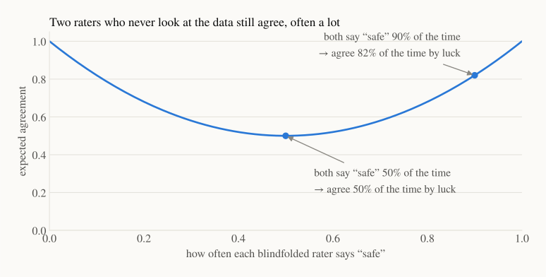
At luck gives 50% agreement. At , which is realistic for safety labels where most responses are fine, luck alone gives 82%. A reported "85% agreement" might mean almost nothing.
2. The common recipe: correct for chance#
Almost every metric in this post has the same shape:
Here is the observed agreement and is the agreement expected by chance. Read it as: of the room above chance (), what fraction did the raters actually use ()?
- 1 means perfect agreement.
- 0 means no better than chance.
- Below 0 means worse than chance: the raters disagree systematically.
The metrics differ mainly in how they estimate . That one choice explains most of their behaviour, including their failures.
3. Cohen's kappa: two raters#
Cohen (1960) estimates chance from each rater's own label frequencies. Here are our two annotators on 50 responses:
| B: safe | B: unsafe | total | |
|---|---|---|---|
| A: safe | 20 | 5 | 25 |
| A: unsafe | 10 | 15 | 25 |
| total | 30 | 20 | 50 |
Observed agreement: the diagonal, .
Chance agreement: A says "safe" 25/50 = 50% of the time, B says it 30/50 = 60% of the time. If they labeled independently, both would say "safe" with probability and both "unsafe" with . In general,
where and are the shares of items that raters A and B put in category . Here , so
The annotators used 40% of the possible room above chance.
How big is big enough?#
The most quoted scale is from Landis and Koch (1977):
| < 0 | 0–0.20 | 0.21–0.40 | 0.41–0.60 | 0.61–0.80 | 0.81–1 | |
|---|---|---|---|---|---|---|
| label | poor | slight | fair | moderate | substantial | almost perfect |
Use it with care: the authors themselves called these divisions arbitrary. Krippendorff (2004) suggests a stricter rule for his : rely on data with , and draw only tentative conclusions when . What counts as "enough" really depends on what you'll do with the labels. A training set can tolerate more noise than a benchmark used to rank models.
Weighted kappa: partial credit for near-misses#
For ordered labels, like a 1–3 helpfulness score, a disagreement between 2 and 3 is milder than one between 1 and 3. Weighted kappa (Cohen, 1968) counts disagreements by how far apart they are:
Here is the observed share of items that rater A put in category and rater B in category . is the share expected by chance, and is the penalty for that disagreement. With ordered categories, linear weights use and quadratic weights use .
Two raters scoring 10 responses on a 1–3 scale:
| Response | 1 | 2 | 3 | 4 | 5 | 6 | 7 | 8 | 9 | 10 |
|---|---|---|---|---|---|---|---|---|---|---|
| Rater A | 1 | 2 | 3 | 3 | 2 | 1 | 3 | 2 | 1 | 2 |
| Rater B | 1 | 3 | 3 | 2 | 2 | 1 | 3 | 1 | 2 | 2 |
Every disagreement here is off by just one step. Plain ignores that, linear weights give , and quadratic weights give . Quadratic weights forgive small slips the most. They are also closely related to the intraclass correlation (Fleiss & Cohen, 1973), which we meet in Section 5.
4. When kappa misbehaves: two paradoxes#
Feinstein and Cicchetti (1990) described two situations where contradicts intuition. Both come from how is computed.
Paradox 1: rare labels sink kappa#
Hold the observed agreement fixed at 90% and change only the prevalence, i.e. how often each rater says "unsafe". The 10% of disagreements are split evenly between the two directions:
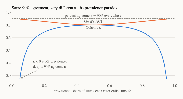
| Prevalence of "unsafe" | 50% | 25% | 10% | 5% |
|---|---|---|---|---|
| Cohen's | 0.80 | 0.73 | 0.44 | −0.05 |
| Gwet's AC1 | 0.80 | 0.84 | 0.88 | 0.89 |
Same 90% agreement, yet falls from "substantial" to "worse than chance". When almost everything is "safe", is already close to 0.9, so there is little room above chance left to earn.
Is wrong? Not exactly. At 5% prevalence, the 5 + 5 disagreements use up every "unsafe" label, so the two raters never agree on a single unsafe response. If unsafe content is what you care about, is sounding a real alarm that 90% agreement hides. The lesson is to always show the confusion table next to the number.
Paradox 2: disagreeing on frequencies raises kappa#
Two pairs of raters, each with 60% agreement on 100 items:
| Pair 1 | Pair 2 | |
|---|---|---|
| Table (rows: A safe/unsafe; columns: B safe/unsafe) | 45, 15 / 25, 15 | 25, 35 / 5, 35 |
| Share labeled "safe" by A, B | 60%, 70% | 60%, 30% |
| 0.54 | 0.46 | |
| Cohen's | 0.13 | 0.26 |
Pair 2's raters have very different habits (60% vs 30% "safe"). That lowers , so goes up: Cohen's rewards systematic bias between raters. Scott's (1955) avoids this by assuming both raters share one pooled label distribution:
For our table in Section 3, the pooled "safe" share is 0.55, so and .
Gwet's AC1: a steadier chance term#
Gwet (2008) argued that the chance term should shrink when one label dominates, because chance agreement only happens when raters are genuinely unsure. With categories and the pooled share of category :
That keeps AC1 near the observed agreement in the paradox figure. It's a useful companion to for skewed data, but not a replacement: as we just saw, 's low value can carry a real message.
5. More than two raters#
Fleiss' kappa#
With raters per item, count agreement as the share of agreeing rater pairs. If of the raters put item in category :
where is the number of items and is the share of all ratings that fall in category . Then .
Despite its name, Fleiss' kappa (1971) generalises Scott's , not Cohen's : it uses pooled frequencies. With two raters it reproduces Scott's exactly (0.394 on our table). It also needs the same number of ratings for every item. In practice that often means throwing away any item with a missing rating.
Krippendorff's alpha#
Krippendorff's flips the view from agreement to disagreement:
is the disagreement we observe between ratings of the same item. is the disagreement we'd expect if all ratings were shuffled across items. ELI5: if mixing the labels up doesn't make disagreement any worse, the raters weren't telling us anything.
It has three practical strengths:
- Any number of raters, and missing ratings are fine. Each item contributes whatever ratings it has.
- Any type of label, through a distance function : nominal (0 if equal, 1 otherwise), ordinal (based on how many ratings fall between the two values), interval () or ratio.
- A small-sample correction. For two raters with no missing data it is almost identical to Scott's (0.400 vs 0.394 on our table).
A worked example with missing ratings
Three raters, six items, labels A/B; "–" means not rated:
| Item 1 | Item 2 | Item 3 | Item 4 | Item 5 | Item 6 | |
|---|---|---|---|---|---|---|
| Rater 1 | A | A | B | A | B | A |
| Rater 2 | A | A | B | B | B | – |
| Rater 3 | A | B | B | – | – | – |
Step 1: the coincidence matrix. Inside each item with ratings, take every ordered pair of ratings from different raters. Each pair adds to the cell for its two values. Item 6 has one rating, so it has no pairs and drops out.
- Item 1 (A, A, A): 6 pairs of (A, A), each worth ½, so gains 3.
- Item 2 (A, A, B): gains 1, gains 1, gains 1.
- Item 3 (B, B, B): gains 3.
- Item 4 (A, B), , each pair worth 1: and each gain 1.
- Item 5 (B, B): gains 2.
Totals: , , . Value counts: , , and pairable ratings.
Step 2: the two disagreements. With the nominal distance, only mismatched cells count:
Step 3: .
Fleiss' kappa can only use the three complete items here (it gives 0.55 on those), throwing away half the data.
How much does that matter? A simulation: 5 raters label 200 items. Each rater is right 85% of the time, 30% of items are truly "unsafe", and each rating goes missing with some probability.
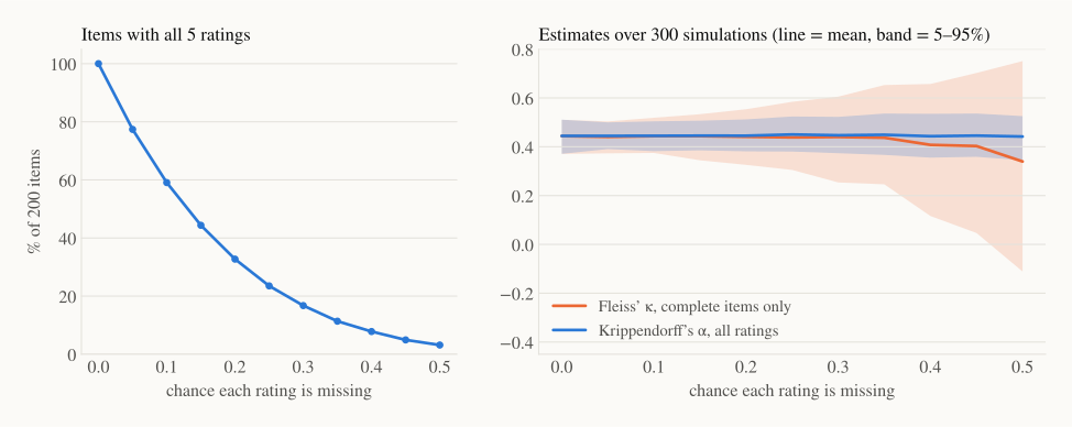
With no missing ratings, the two give the same answer (0.44). At a 30% chance of missing, only 17% of items still have all five ratings. Fleiss' estimate then swings between 0.25 and 0.61 across simulations, while stays between 0.37 and 0.52 because it still uses every rating.
Continuous scores: the intraclass correlation#
For numeric ratings, like a 0–100 quality score, the usual tool is the intraclass correlation (ICC). It is the share of the score's variance that comes from real differences between items rather than from raters or noise. There are several versions (Shrout & Fleiss, 1979): whether raters are a random sample or fixed, and whether you care about one rater or the average of several. Always state which one you report. Krippendorff's with the interval distance is an alternative that also tolerates missing ratings.
6. In practice: humans, LLM judges and honest reporting#
LLM-as-a-judge. When an LLM grades model outputs, its agreement with humans should be compared with human–human agreement on the same items, since that is the realistic ceiling. Zheng et al. (2023) reported that strong LLM judges such as GPT-4 reach over 80% agreement with human preferences, the same level as humans agree with each other. That is percent agreement; given everything above, it's worth also reporting a chance-corrected number.
Agreement is not accuracy. Two judges who share the same blind spot, say an LLM judge and annotators who both prefer longer answers, can agree perfectly and both be wrong. Agreement measures consistency. To measure correctness you need a reference: expert labels, or items whose answer is known.
Report uncertainty. With 50 items, our has a 95% bootstrap interval of [0.14, 0.64], from resampling items with replacement 5,000 times. That interval stretches from "slight" to "substantial", so a single number without an interval says much less than it seems.
Choosing a metric:
| Situation | Start with |
|---|---|
| 2 raters, categories, balanced classes | Cohen's , plus percent agreement |
| Ordered scores (1–5) | weighted (quadratic) or ordinal |
| 3+ raters, everyone rates every item | Fleiss' or |
| Missing ratings, crowdsourcing, varying raters | Krippendorff's |
| Rare labels (e.g. 5% unsafe) | and AC1, plus the confusion table |
| Continuous scores | ICC (state the form) or interval |
7. In code#
import numpy as np
import krippendorff
from sklearn.metrics import cohen_kappa_score

# Section 3: 50 responses, 0 = safe, 1 = unsafe
a = np.array([0] * 25 + [1] * 25)
b = np.array([0] * 20 + [1] * 5 + [0] * 10 + [1] * 15)
print(f"Cohen's kappa = {cohen_kappa_score(a, b):.2f}")

# Section 5: 3 raters x 6 items, A = 0, B = 1, nan = no rating
nan = np.nan
ratings = np.array([[0, 0, 1, 0, 1, 0],
                    [0, 0, 1, 1, 1, nan],
                    [0, 1, 1, nan, nan, nan]])
alpha = krippendorff.alpha(reliability_data=ratings, level_of_measurement="nominal")
print(f"Krippendorff's alpha = {alpha:.2f}")
Cohen's kappa = 0.40
Krippendorff's alpha = 0.43
8. Where it breaks#
- One number hides the structure. The same can come from evenly spread disagreements or from raters who never agree on the rare class. Always look at the confusion table.
- Thresholds are conventions. "0.6 is substantial" is a rule of thumb, not a law. Decide what your downstream use needs.
- Prevalence moves the goalposts. Two datasets with different label balance can't be compared on alone.
- Too few items. Agreement on 30 items comes with an interval wide enough to make most comparisons meaningless.
- Unclear guidelines look like bad raters. Low agreement is often a sign that the labeling instructions are ambiguous. Fix those before blaming the annotators (or the LLM judge).
Recap#
- Percent agreement rewards luck. Two raters who both say "safe" 90% of the time agree 82% of the time without looking.
- Chance-corrected metrics share one formula, , and differ in how they estimate chance agreement .
- Cohen's uses each rater's own frequencies: agreement became in our example. Weighted gives partial credit on ordered scales.
- paradoxes: rare labels can push below zero at 90% agreement, and rater bias can raise it. Report AC1 and the confusion table alongside it.
- Fleiss' extends Scott's to many raters. Krippendorff's handles any number of raters, missing ratings and any label type.
- For LLM judges: compare against human–human agreement, report intervals, and remember that agreement is not accuracy.