
LLM Interpretability, Layer by Layer — Part 1: Reading the Residual Stream
November 7, 2026 · 5 min read · Interpretability, Large Language Models, Machine Learning
In Part 0 we met the residual stream: one vector per token that every layer reads and adds to, ending in a prediction for the next token. This post takes the simplest possible look inside. Read the stream at every layer and ask what it "says."
This is the first rung of the ladder, observe. By the end you'll know:
- the logit lens, a one-line trick to decode any layer,
- what it shows for "Michael Jordan plays the sport of",
- how to read attention patterns,
- why neither one, on its own, explains anything.
1. The logit lens#
The model turns its final residual vector into a prediction with two steps: a normalization (ln_final) and the unembedding matrix , which gives a score to each of the 50,257 tokens:
The logit lens (nostalgebraist, 2020) applies the same two steps to the residual stream at an earlier layer:
It asks: if the model had to answer right now, at layer , what would it say?
Why should this work at all? Because of the running sum from Part 0. Every layer adds to the stream; no layer replaces it. The last layer's output is just the earlier stream plus a few more additions. So if the answer is being built up gradually, early versions of it should already point in roughly the right direction.
ELI5: a student writes an essay draft by draft, never deleting, only adding. The logit lens reads each draft as if it were the final version. Early drafts are rough, but you can watch the main argument appear.
import torch
from transformer_lens.model_bridge import TransformerBridge

torch.set_grad_enabled(False)
model = TransformerBridge.boot_transformers("gpt2", device="cpu")
model.enable_compatibility_mode()

prompt = "Michael Jordan plays the sport of"
logits, cache = model.run_with_cache(prompt)
target = model.to_single_token(" basketball")

for layer in range(12):
    x = cache[f"blocks.{layer}.hook_resid_pre"][:, -1:]       # stream at the last token, before layer
    probs = model.unembed(model.ln_final(x))[0, -1].softmax(-1)
    rank = (probs > probs[target]).sum().item() + 1
    print(f"layer {layer:2d}: top = {model.to_string(probs.argmax())!r:14}  "
          f"P(basketball) = {probs[target]:.3f}  rank = {rank}")
# layer  0: top = ' destro'       P(basketball) = 0.000  rank = 39677
# layer  6: top = ' course'       P(basketball) = 0.008  rank = 9
# layer  8: top = ' baseball'     P(basketball) = 0.135  rank = 3
# layer  9: top = ' basketball'   P(basketball) = 0.425  rank = 1
# layer 10: top = ' basketball'   P(basketball) = 0.949  rank = 1   (selected lines)
2. Watching the answer form#
Here is the logit lens on every token and every layer at once. Each cell shows the most likely next token if the model stopped there, and the shade shows how confident it is:
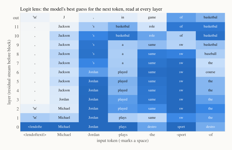
A few things to notice:
- The bottom row just repeats the input. At layer 0, the stream is the token's embedding, and GPT-2 uses the same matrix to embed and unembed tokens, so the lens mostly reads the token back.
- The last column is the one that matters. After
of, the guess goes through the generic "the" in the early layers, then "course" (as in "of course"), "baseball" at layer 8, and finally "basketball" from layer 9 on. - Other positions make their own guesses. After
Michael, the model predicts "Jackson": the most famous Michael in its training data. Afterplays, layers 10 and 11 already predict "basketball": the model has guessed where the sentence is going.
The probability and rank of " basketball" at the last token tell the same story more precisely:
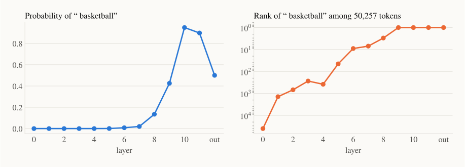
The rank climbs steadily, from 39,677th at layer 0 to the top 10 by layer 6 and first place at layer 9. The probability only becomes visible late: 1% at layer 6, 14% at layer 8, then 95% at layer 10. Notice the drop at the end: the final layers take probability away from basketball (95% → 50%) and spread it over football, golf and others. Models often do this. The last layers seem to calibrate how sure the model sounds, not just pick the answer.
What the lens can't do. It assumes every layer "speaks the same language" as the output. That isn't quite true, especially in early layers, which is why the bottom rows are mostly noise. The tuned lens (Belrose et al., 2023) fixes this by training a small linear translator for each layer. For GPT-2 small, the plain logit lens is good enough to see the shape of the story.
3. Attention patterns#
The logit lens shows what the stream says. Attention patterns show where information moves. For each head, the pattern is a table: for every token (row, the query), how much it reads from every earlier token (column, the key). Each row adds up to 1.
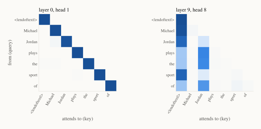
The left head (layer 0, head 1) mostly looks at the token itself. The right head (layer 9, head 8) is more interesting. From the last token of, it puts 59% of its attention on Jordan. That fits a story: the sport is attached to the name, and this head carries it to the end of the sentence, where the answer is needed. (I picked this head because it attends most from the last token to Jordan, so its existence isn't a surprise. The question is whether it matters.)
Notice also how much attention goes to the first token, <|endoftext|>. Many heads use the first position as a "nothing to do" spot: when a head has nothing useful to read, its attention collects there.
4. Why this isn't an explanation yet#
It's tempting to stop here: "Layer 9, head 8 moves 'Jordan' to the end, and basketball appears at layer 9. Mystery solved." But look at what we actually showed:
- The logit lens shows a correlation in time. Basketball becomes readable around layer 9. That doesn't tell us which component put it there. Many heads and MLPs write to the stream at every layer.
- Attention shows where a head looks, not what it carries. A head can attend strongly to
Jordanand copy something irrelevant, or copy nothing useful. A head that attends weakly can still carry the key information. - Choosing what to show is itself a bias. I chose the head that best fit the story. With 144 heads, some head will usually fit any story.
This is the observe rung. It's great for forming a hypothesis: the fact lives at the athlete's name, and late-layer attention moves it to the last token. Testing that hypothesis needs stronger tools. Part 4 will test it directly, and it will turn out to be mostly right, with some surprises.
Recap#
- The logit lens decodes the residual stream at any layer with the model's own final normalization and unembedding. It works because every layer adds to the stream.
- For "Michael Jordan plays the sport of," basketball's rank climbs steadily, reaches first place at layer 9 and peaks at 95% at layer 10. The last layers then lower its probability to 50%.
- Attention patterns show where each head reads from. Head 9.8 moves attention from the last token to
Jordan. - Both are observations. They suggest where to look, but they can't tell us which parts cause the answer.
Next up — Part 2: Probes and Linear Directions. Instead of reading the stream through the model's own output layer, we train our own small readers, called probes, to ask a direct question: is "this athlete plays basketball" written in the stream, and where? We also meet the most common way probes fool you.