
LLM Interpretability, Layer by Layer — Part 2: Probes and Linear Directions
November 7, 2026 · 6 min read · Interpretability, Large Language Models, Machine Learning
In Part 1 we read the residual stream through the model's own output layer. That only shows information the model is about to say. But the stream carries much more: what the sentence is about, who is being mentioned, what kind of word comes next. To read that, we build our own readers.
A probe is a small classifier trained to predict some property from the model's internal activations. If a simple probe can read "this athlete plays basketball" from the stream at layer 6, the information is there, in a usable form.
This is the correlate rung of the ladder. By the end you'll know:
- how to train a linear probe and what its accuracy means,
- the linear representation hypothesis,
- where GPT-2 stores an athlete's sport,
- the baselines and controls without which probe results are easy to misread.
1. A probe is just a classifier on activations#
We need a dataset where we know the answer. Ours is 120 famous athletes, 30 each from basketball, baseball, American football and golf. For each one, we run "[name] plays the sport of" through GPT-2 and save the residual stream at every layer, at two positions: the athlete's last name token and the last token of.
Then, for each layer separately, we train a linear probe: multinomial logistic regression from the 768-dimensional vector to the four sports,
We always report accuracy on held-out athletes (5-fold cross-validation), never on athletes the probe was trained on. With 768 dimensions and only 96 training athletes per fold, a probe could otherwise just memorize them.
Why linear? Because a powerful enough probe (a deep network) could compute the answer itself from the athlete's name, and then we'd be measuring the probe, not the model. A linear probe can only read information that is already laid out simply.
ELI5: you want to know whether a student understood a lecture. A short quiz (a linear probe) tells you what they took in. Giving them a textbook and a week to study (a powerful probe) only tells you how good the textbook is.
2. The linear representation hypothesis#
Linear probes work surprisingly well across many models and concepts, and that's a finding in itself. The linear representation hypothesis says that models store many concepts as directions in activation space. "Plays basketball" corresponds roughly to some vector , and the more an activation points along , the more the model "believes" it.
If that's true, there's an even simpler probe than logistic regression: the difference of means. Average the activations of all basketball players, average those of all golfers, and subtract:
The projection then scores how basketball-like versus golf-like an athlete looks. These directions come back in Part 6, where we add them to the stream to change the model's answer.
3. Where is "which sport" stored?#
Here are held-out probe accuracies at every layer:
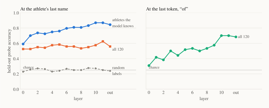
There's a lot in this figure, so let's go line by line.
Right panel, at the last token of. The probe starts near chance (31% at layer 0; chance is 25%) and climbs to 70% at layers 10–11. That fits Part 1: the sport only arrives at the last position late in the network.
Left panel, at the athlete's name. Two surprises.
First, the orange line (all 120 athletes) is already at 52% at layer 0, well above chance, before the model has done any processing. Layer 0 is just the embedding of the last-name token. The probe is reading clues from the name itself: some surnames are more common among baseball players of a certain era, some among golfers, and so on. This is our first baseline lesson. Always check the probe at layer 0. Whatever it gets there comes from the input, not from the model's knowledge.
Second, for all 120 athletes, the line barely rises (52% → 62% at best). That's because GPT-2 small doesn't know many of them. When we ask the model itself, comparing its scores for the four sport words, it picks the right sport for only 69% of the athletes, and that is after correcting for its general preference for "football" and "basketball". Without the correction, it answers golf for only 2 of the 30 golfers. You can't read knowledge from the stream that isn't there.
Restricted to the 83 athletes the model knows (blue line), the picture becomes clear. Accuracy rises from 59% at layer 0 to 80% by layer 6 and 87% at layers 10–11. The extra accuracy over layer 0 is what the model's own layers added: the sport is being looked up at the athlete's name in the early and middle layers. (Part 4 will show that the first MLP layers do most of this lookup.)
4. Keeping probes honest#
The grey dashed line is a control task (Hewitt and Liang, 2019). Each athlete gets a random "sport", fixed for that athlete, and we train the same probe to predict it. A probe that's too powerful could learn arbitrary labels. Ours stays at chance (23%–28%) on every layer, so it isn't just memorizing.
Here is a checklist for reading any probe result:
- Held-out data only. Report accuracy on examples the probe never saw. With high-dimensional activations and small datasets, training accuracy is meaningless.
- A layer-0 or input baseline. What can be read from the input alone? Here, 52% came from surnames.
- A control task or random-label baseline. Can the probe learn nonsense just as well?
- Condition on what the model knows. Probing for knowledge the model lacks only measures noise.
- Remember the rung. A probe shows information is present and linearly readable. It doesn't show the model uses it. A model could store a fact and then never look at it again.
The fifth point matters most. Here's a direct way to see it. Below, the athletes are projected onto two kinds of 2-D views at layer 8:
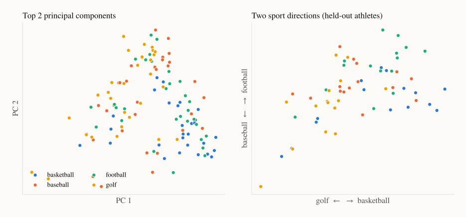
On the left, the top two principal components (the directions of largest variance) show no clear grouping by sport. The biggest differences between athletes' activations are about other things, such as how the name is tokenized or how famous it is. On the right, we project onto two difference-of-means directions (golf → basketball and baseball → football). To keep it honest, the directions were computed from half the athletes, and the plot shows only the other half. Basketball players drift to the right and football players to the top, though the groups overlap a lot.
The lesson: "sport" is a small, specific direction in a 768-dimensional space, not the main thing the stream encodes. You find it by asking for it with labels, and that's exactly why you then have to check that the model uses it.
5. In code#
import numpy as np
from sklearn.linear_model import LogisticRegression
from sklearn.model_selection import StratifiedKFold, cross_val_score

# ATHLETES = {"basketball": ["Michael Jordan", ...], "baseball": [...], ...}  (120 names)
X, y = [], []
for k, (sport, people) in enumerate(ATHLETES.items()):
    for person in people:
        _, cache = model.run_with_cache(f"{person} plays the sport of")
        pos = len(model.to_str_tokens(person)) - 1               # last token of the name
        X.append(np.stack([cache[f"blocks.{l}.hook_resid_pre"][0, pos].numpy() for l in range(12)]))
        y.append(k)
X, y = np.stack(X), np.array(y)                                  # [athletes, layers, 768]

cv = StratifiedKFold(5, shuffle=True, random_state=0)
for layer in [0, 6, 11]:
    probe = LogisticRegression(C=0.1, max_iter=5000)
    acc = cross_val_score(probe, X[:, layer], y, cv=cv).mean()
    control = cross_val_score(probe, X[:, layer], np.random.default_rng(0).permutation(y), cv=cv).mean()
    print(f"layer {layer:2d}: probe {acc:.2f}   random labels {control:.2f}")
# layer  0: probe 0.53   random labels 0.17
# layer  6: probe 0.56   random labels 0.23
# layer 11: probe 0.62   random labels 0.26
Any list of well-known players works: we used 30 per sport, chosen before looking at the model's answers.
Recap#
- A probe is a simple classifier on internal activations. Linear probes only read what is already laid out simply, so they say something about the model, not the probe.
- The linear representation hypothesis: many concepts are directions in activation space. A difference of means between two groups gives such a direction cheaply.
- In GPT-2 small, an athlete's sport becomes readable at the athlete's name during the early and middle layers (87% for athletes the model knows), and at the last token only in layers 10–11 (70%).
- Baselines matter: the surname alone gave 52% at layer 0, and random labels gave about 25%.
- Probes reach the correlate rung. They show information is present, not that it is used.
Next up — Part 3: Superposition and Sparse Autoencoders. We needed labels to find the sport direction. Could we find meaningful directions without labels? Single neurons turn out to be a poor place to look, for an interesting reason called superposition. Sparse autoencoders find features in GPT-2 that track sports, LaTeX math, and more.