
LLM Interpretability, Layer by Layer — Part 4: Causal Validation with Activation Patching
November 7, 2026 · 7 min read · Interpretability, Large Language Models, Machine Learning
Parts 1 to 3 gave us a consistent story through observation and correlation. An athlete's sport is looked up at the athlete's name in the early and middle layers, then moved to the last token in the late layers, where the answer is produced. But every piece of evidence so far was a correlation. The information is there, but is it used?
This post climbs to the cause rung. The idea is simple and powerful: change one internal activation and see whether the output changes. By the end you'll know:
- how to set up a clean and a corrupted run, and score the difference,
- activation patching, the core causal tool of mechanistic interpretability,
- what patching shows about how GPT-2 recalls an athlete's sport,
- attribution patching, a fast approximation, and the pitfalls of both.
1. Clean, corrupted, and a metric#
We need two prompts that differ in exactly one detail, the detail we care about:
- clean: "Kobe Bryant plays the sport of" → basketball,
- corrupted: "Tiger Woods plays the sport of" → golf.
Both prompts have the same number of tokens in the same roles: two first-name pieces, a last name, then plays the sport of. That way "position 3" means "the last name" in both. (We switch from Michael Jordan to Kobe Bryant for exactly this reason: GPT-2 splits Tiger into two tokens, like Kobe, but Michael is one.)
To score how much the model prefers basketball, we use the logit difference:
It's 4.29 on the clean prompt and −3.69 on the corrupted one. Logit differences are better than probabilities here because they are on the scale where the model adds things up (the residual stream adds contributions, and logits are linear in it), and they compare the two answers we care about while ignoring everything else.
2. Activation patching#
Here's the experiment, called activation patching (also called causal tracing or interchange intervention):
- Run the clean prompt and save every activation.
- Run the corrupted prompt, but at one chosen place (say, the residual stream at layer 5, position 3), replace the activation with the saved clean one.
- Measure the logit difference, and report it as the share of the answer restored:
A score of 1 means this single activation carries everything needed to bring back "basketball." A score of 0 means it carries nothing that matters for this difference.
ELI5: two cars, one runs and one doesn't. You swap one part at a time from the good car into the broken one. When the broken car starts, you've found a part that matters. Unlike watching the engine (observing), swapping parts tells you what causes the difference.
This direction, running the corrupted prompt and patching in clean activations, is called denoising. It asks: is this activation enough to restore the behaviour? The opposite, noising, runs the clean prompt and patches in corrupted activations. It asks: is this activation needed? They can disagree, for example when two parts each carry a full copy of the information (each is sufficient, neither is necessary). Here we use denoising.
3. Where the fact lives, causally#
We patch every layer and every position, in three places: the residual stream, the attention outputs and the MLP outputs. To avoid relying on one example, we average over four basketball players with the same token structure (LeBron James, Kobe Bryant, Wilt Chamberlain, Kyrie Irving), each against Tiger Woods. (GPT-2 small clearly prefers golf for only two golfers, Tiger Woods and Jack Nicklaus, and only Tiger Woods is split into tokens the same way as these basketball players.)
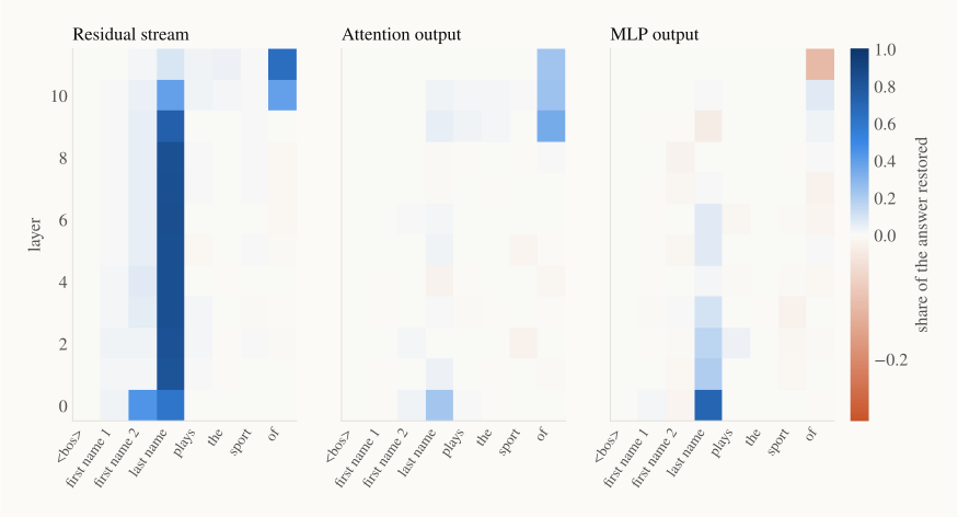
Residual stream (left). A bright column at the last-name token: patching the clean stream there restores about 84% of the answer at every layer from 1 to 8. Then the effect fades at the name (74% at layer 9, 39% at layer 10) and appears at the last token (39% at layer 10, 65% at layer 11). Nothing else matters: patching plays, the or sport does nothing, since those words are the same in both prompts.
This is the story from Parts 1–3, now confirmed causally: the sport is at the name until layer 9, and then it moves to the end.
MLP outputs (right). Who writes the sport at the name? Mostly the layer-0 MLP, which alone restores 71%. Layers 1–3 add smaller amounts (19%, 16% and 10%). The early MLPs act as a lookup table: given the tokens of a name, write the associated facts into the stream. This fits a larger body of work on factual recall, which finds facts stored in early-to-middle MLPs at the subject's last token (Meng et al., 2022). In GPT-2 small, the lookup happens strikingly early.
Attention outputs (middle). Who moves the sport to the end? Attention at the last token in layers 9, 10 and 11 (restoring 34%, 24% and 23%). That's where head 9.8 from Part 1 lives. Its attention from the last token to the name now has a causal partner: the attention output there carries the answer.
One more detail: the MLP at the last token in layer 11 has a negative score (−11%). Patching it in makes the model less sure of basketball. This matches what Part 1's logit lens showed, where the last layer lowered basketball's probability from 90% to 50%. Some components push against the answer, as a kind of calibration.
4. In code#
model = ...  # TransformerBridge GPT-2, as in Part 0
clean, corrupt = "Kobe Bryant plays the sport of", "Tiger Woods plays the sport of"
b, g = model.to_single_token(" basketball"), model.to_single_token(" golf")
ld = lambda logits: (logits[0, -1, b] - logits[0, -1, g]).item()

clean_logits, clean_cache = model.run_with_cache(clean)
ld_clean, ld_corrupt = ld(clean_logits), ld(model(corrupt))

def restored(layer, pos):
    def patch(act, hook):
        act[:, pos] = clean_cache[hook.name][:, pos]          # swap in one clean activation
        return act
    out = model.run_with_hooks(corrupt, fwd_hooks=[(f"blocks.{layer}.hook_resid_pre", patch)])
    return (ld(out) - ld_corrupt) / (ld_clean - ld_corrupt)

print(f"clean {ld_clean:.2f}, corrupted {ld_corrupt:.2f}")
for layer, pos, where in [(4, 3, "last name"), (4, 7, "last token"), (11, 3, "last name"), (11, 7, "last token")]:
    print(f"layer {layer:2d}, {where:10s}: {restored(layer, pos):.2f}")
# clean 4.29, corrupted -3.69
# layer  4, last name : 0.77
# layer  4, last token: 0.02
# layer 11, last name : 0.08
# layer 11, last token: 0.66
For Kobe Bryant alone the numbers are a little different from the four-player average in the figure (77% rather than 84% at the name), but the pattern is the same.
5. A faster approximation: attribution patching#
Activation patching needs one forward pass per activation you test. That's fine for 12 layers × 8 positions, but a modern model has tens of layers, thousands of positions and many components. Attribution patching (Nanda, 2023) estimates every patch at once with a first-order Taylor expansion:
One forward and one backward pass on the corrupted prompt gives the gradient at every activation . One forward pass on the clean prompt gives every . A dot product then estimates every patch.
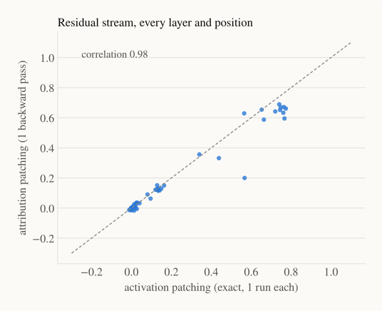
For the residual stream on Kobe vs Tiger, the estimates correlate 0.98 with the exact results. They are least accurate for the biggest effects, where the linear approximation breaks down (several points near 0.75 are estimated at about 0.65). The practical recipe: use attribution patching to search, then confirm the important findings with exact patching.
6. Pitfalls#
Patching is the workhorse of causal interpretability, and it has well-known traps:
- The corruption defines the question. Kobe → Tiger asks "what distinguishes basketball from golf?" Corrupting with random noise, or with a made-up name, asks different questions and can give different maps. Choose the corruption that matches what you want to explain.
- Patches can push activations off-distribution. Mixing parts of two runs can create combinations the model never saw in training, so a component can look important just because the mix confused the model. Patching between two natural prompts, as we did, reduces this.
- Denoising and noising answer different questions (sufficient vs necessary), as explained above. Report which one you used.
- Positions must line up. If the prompts tokenize differently, "position 3" means different things in each run. That's why we chose names with the same token structure.
- A heatmap is not a mechanism. We know where the answer is computed: early MLPs at the name, late attention at the end. We don't yet know how those parts work together. Mapping that is the job of a circuit, in the next part.
Recap#
- Activation patching: run a corrupted prompt, swap in one activation from a clean run, and measure how much of the clean behaviour comes back. It tests cause, not just correlation.
- Score with the logit difference between the two competing answers, normalized to "share restored."
- For athlete → sport in GPT-2 small: the layer-0 MLP at the athlete's last name writes most of the sport (71%), the stream carries it at the name through layer 8, and attention at the last token in layers 9–11 moves it to where the answer is produced. This confirms the earlier observations.
- Attribution patching estimates all patches in one backward pass (correlation 0.98 with the exact results here). Use it to search, then confirm with exact patching.
- Patching shows where, not how.
Next up — Part 5: Mechanisms, Finding a Circuit. We map a full mechanism: how GPT-2 completes "When Mary and John went to the store, John gave a drink to" with Mary. It's one of the best-studied circuits in any language model, with distinct teams of attention heads, a surprising self-repair, and a lesson about what "the circuit" really means.