
LLM Interpretability, Layer by Layer — Part 3: Superposition and Sparse Autoencoders
November 7, 2026 · 7 min read · Interpretability, Large Language Models, Machine Learning
In Part 2 we found a "sport" direction, but only because we went looking for it with labelled data. That approach has a built-in limit: you can only find concepts you already thought of. The model may represent thousands of things nobody would think to probe for.
Can we find meaningful directions without labels? The obvious place to start is the model's neurons, the individual numbers inside each MLP. This post explains why neurons disappoint, and what works better.
This is still the correlate rung, now without labels. By the end you'll know:
- why neurons are often polysemantic (one neuron, many unrelated meanings),
- superposition: how a model stores more features than it has dimensions,
- sparse autoencoders (SAEs), which pull those features back out,
- what SAE features look like in GPT-2, and how to check that they mean what you think.
1. One neuron, many meanings#
If each neuron stood for one concept ("basketball", "French text", "a closing bracket"), interpretability would be easy: list the neurons and label them. Early vision research found some neurons like that. But in language models, most neurons are polysemantic. A single neuron might fire on academic citations, Korean text, and HTTP requests. Its label would be a list of unrelated things.
Why would a network do something so confusing? Because of a mismatch in numbers. GPT-2 small has 768 dimensions in its residual stream and 3,072 neurons per MLP layer. The number of concepts it needs (every name, topic, grammatical role and writing style) is far larger.
2. Superposition: more features than dimensions#
The key fact is that most features are rare. In any given sentence, almost none of the millions of possible concepts are present. A sentence about basketball rarely also involves cooking, Python code and Korean grammar at the same time.
Elhage et al. (2022) showed what a network does with that in a tiny experiment. Take 5 features, each present only now and then, and force the network to squeeze them into 2 dimensions and then reconstruct them:
Each column of is the 2-D direction where one feature is stored. Here is what training finds, depending on how often features appear:
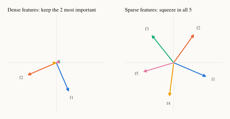
When features are dense (all present at once, left), the network keeps the 2 most important features at right angles and drops the other 3. That's what you'd expect: 2 dimensions, 2 features.
When features are sparse (each present only 10% of the time, right), the network stores all 5, spread out like a pentagon. The directions aren't at right angles, so they interfere. But since two features are rarely active together, the interference rarely matters, and the ReLU filters out the small leftover noise. Storing more features is worth a little noise.
That's superposition: a network represents more features than it has dimensions, by giving them almost-but-not-quite independent directions. In 768 dimensions, there's room for a huge number of nearly-at-right-angles directions. The cost is that no single neuron lines up with a single feature, which is why neurons look polysemantic.
ELI5: a small apartment with one closet. If you need your winter coat and your swimsuit at different times of year, you can hang them on the same hook. You'd only have a problem if you needed both on the same day, and that rarely happens.
3. Sparse autoencoders: unmixing the features#
If features are stored as directions in superposition, we need a way to find those directions. A sparse autoencoder (SAE) does this. It is a second, much wider network trained to rebuild the model's activations through a bottleneck that is wide but sparse:
trained to minimize
Here is the residual stream (768 numbers), has many more entries (24,576 for the SAE we use), and the term pushes most of them to exactly zero. Each column of is a candidate feature direction, and says how strongly feature is present.
The bet is that the cheapest way to rebuild activations from a few active features at a time is to discover the features the model actually uses. No labels are needed.
We use a pretrained SAE for GPT-2 small, trained by Joseph Bloom on the residual stream before layer 8 (gpt2-small-res-jb in SAELens). On 75,870 tokens of this blog's own posts, it uses 72 active features per token on average, out of 24,576, and rebuilds 78% of the variance of the residual stream. On a sample of text, swapping the SAE's reconstruction into the model raises the next-token loss from 4.25 to 4.41. Something is lost, but most of the model's behaviour survives.
4. What the features look like#
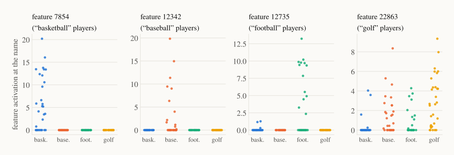
Found from sports. Without training anything new, we run the 120 athletes from Part 2 through the SAE and, for each sport, look for the feature that fires most selectively on that sport's players (at the last-name token):
| Feature | Fires on its own sport | Fires on the other three |
|---|---|---|
| 7854 ("basketball player") | 67% | 0% |
| 12342 ("baseball player") | 40% | 0% |
| 12735 ("football player") | 43% | 3% |
| 22863 ("golf"?) | 83% | 36% |
Three of the four are remarkably clean. Feature 7854 fires on two thirds of basketball players and never on any other athlete. This is what Part 2's sport direction looked like with labels, now found without them. The golf feature is much less selective, which fits what we've seen all along: GPT-2 small barely knows golfers.
Found from this blog. The SAE also finds features for things on this blog that nobody would think to probe for. For each feature, the most useful thing to look at is the text where it fires most strongly. Here are two features: one that fires much more in LaTeX math than in plain text, and one that fires more in Python code. The highlighted token is where the feature fires, and the number is its activation:
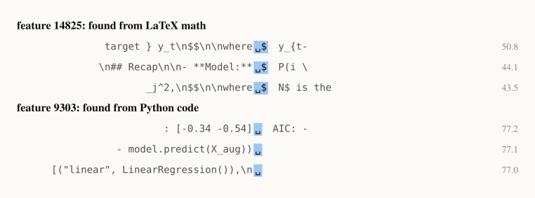
Feature 14825 is a clean "opening dollar sign of inline math" feature: it fires on $ right before LaTeX like y_{t-1} or P(i.
Feature 9303 is a cautionary tale. I found it by asking which feature fires most in Python code, and expected something like "code" or "function call". Its top examples show what it really responds to: a lone space token, the kind that appears in aligned code and in tables. It is about whitespace, not code. Looking at the top activations corrected a label that the selection method suggested.
5. How to check a feature#
SAE features are hypotheses, not facts. Before believing a label:
- Look at many top activations, not one. Feature 9303 looked like "code" until we looked.
- Look across the activation range, not just the top. A feature can mean "basketball" at its peak and something vaguer at low values.
- Check the corpus. On this blog, which has no sports, feature 7854's strongest activation was 3.1 (on the word ridge); on basketball players it reached 20. What a feature looks like depends heavily on what text you run.
- Check the reconstruction. Features from an SAE that only rebuilds 78% of the variance miss the other 22%. Some of the model's computation lives in what the SAE leaves out.
- Test it causally. A feature that tracks a concept still might not be used. That's the next rung, and Part 6 shows how to steer with feature-like directions.
Two more known issues. Feature splitting: a bigger SAE may split "basketball player" into "NBA star", "college basketball", and so on, so "the" feature for a concept depends on the SAE's size. Absorption: a general feature can lose some cases to a more specific feature that takes over, making the general one look less reliable than it is. Neither makes SAEs useless, but both are reasons to treat features as useful approximations, not the model's true parts.
6. In code#
from sae_lens import SAE

sae = SAE.from_pretrained(release="gpt2-small-res-jb", sae_id="blocks.8.hook_resid_pre", device="cpu")

_, cache = model.run_with_cache("Kobe Bryant plays the sport of")
x = cache["blocks.8.hook_resid_pre"][0]          # [position, 768]
f = sae.encode(x)                                # [position, 24576], mostly zeros
name_pos = 3                                     # <|endoftext|>, K, obe, " Bryant"
print("active features at ' Bryant':", (f[name_pos] > 0).sum().item())
print("basketball feature 7854:", round(f[name_pos, 7854].item(), 1))
print("top features:", f[name_pos].topk(5).indices.tolist())
# active features at ' Bryant': 48
# basketball feature 7854: 5.9
# top features: [5555, 12472, 13526, 5009, 19016]
Feature 7854 is active but not among the top five: the strongest features at a name are usually about other things, such as "this is a person's surname" or "famous person". The sport is one small part of what the stream says about Kobe Bryant.
Websites such as Neuronpedia show top activations and explanations for every feature of many public SAEs, including this one (gpt2-small/8-res-jb).
Recap#
- Most neurons are polysemantic because of superposition: models store far more features than they have dimensions, as nearly-independent directions, which works because most features are rarely active.
- A sparse autoencoder rebuilds activations from a wide, sparse set of features. Its decoder columns are candidate feature directions, found without labels.
- On GPT-2 small (layer 8), the SAE finds features for basketball, baseball and football players that are almost perfectly selective, and features for LaTeX math, but a "code" feature turned out to be a whitespace feature.
- Check features by reading many examples, across the activation range and corpus, and by testing them causally.
Next up — Part 4: Causal Validation with Activation Patching. We now have plenty of correlations: the logit lens, probes and SAE features all point to the athlete's name in early-to-middle layers, and to the last token late. Time to climb a rung. We'll swap activations between two runs, Kobe Bryant and Tiger Woods, and measure exactly which parts of the model cause the answer.