
Conformal Prediction, Step by Step — Part 1: Split Conformal, the Whole Trick
November 7, 2026 · 6 min read · Conformal Prediction, Uncertainty Quantification, Machine Learning, Statistics
In Part 0 we saw the core idea: measure a model's errors on data it has never seen, and use them to size the range around each prediction. This post turns that idea into a precise method, split conformal prediction, and answers the question every reader should ask: why should the 90% promise actually hold?
By the end you will know:
- the three-step recipe, written out exactly,
- where the strange in the quantile comes from (a five-line proof),
- how it works on a real dataset,
- what "90% coverage" really means, checked by running it a thousand times.
1. The recipe#
We start with a labelled dataset and split it into two parts:
- a training set, used to fit any model we like;
- a calibration set , which the model never sees during training.
Then we follow the three steps from Part 0.
Step 1: score. For each calibration point, measure how wrong the model is:
This is the score (often called the nonconformity score: how much a point fails to "conform" to the model). Bigger means worse.
Step 2: quantile. Sort the scores and pick the -th smallest, where
Here means the -th smallest score, and rounds up. With and , we get : the 901st smallest of the 1000 scores, a bit above the plain 90% quantile.
Step 3: keep. For a new input , keep every answer whose score would be at most :
That's it. One model fit, one sort, one number , used for every new point.
Here are steps 1 and 2 on the toy data from Part 0, using a random forest trained on 300 other points:
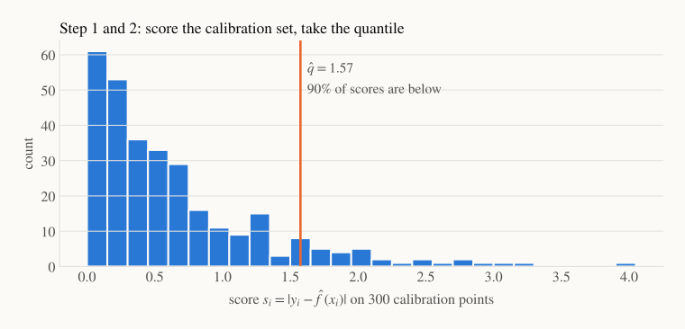
Most points have small errors and a few have large ones. The orange line marks , so every prediction gets the band . That band is the one in the right panel of Part 0's figure.
2. Why it works: the rank argument#
The guarantee is that, for a new point ,
The proof needs no calculus, only one idea about ranks.
Let be the score of the new point. The new point is inside the interval exactly when , so we need to show that .
Now use exchangeability. The model was trained on separate data, so it treats the calibration points and the new point the same way. The scores are therefore exchangeable: no score is special, so the new score is equally likely to be the smallest, the second smallest, …, or the largest of the . (We assume no ties for simplicity; ties only make coverage higher.)
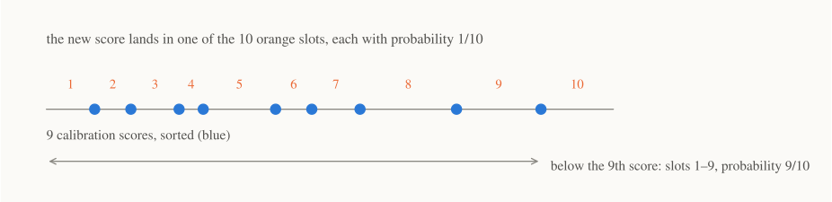
With 9 calibration scores there are 10 slots, and the new score lands in each with probability . It is below the 9th score in 9 of the 10 slots. In general, the new score falls at or below the -th smallest calibration score with probability
We want this to be at least , so we need . The smallest such whole number is . That is exactly the from step 2, and the proof is done.
Why and not ? Because there are scores in the game: the we have and the one we are about to see. The correction matters most when is small. With and :
- the corrected rule picks , so coverage is , as promised;
- the naive rule picks , so coverage is , well short of 90%.
If comes out larger than (for 90%, that happens when ), we don't have enough calibration data to promise 90%, and the honest answer is an infinitely wide interval.
The same argument also gives an upper bound. Without ties, coverage is at most , so with 1000 calibration points we get between 90% and 90.1%. Conformal intervals aren't needlessly wide.
3. A real example: California house prices#
Let's try it on real data. The California Housing dataset has 20,640 neighbourhoods. The features are things like median income, house age and location, and the target is the median house price, in units of $100,000. We split it 50/25/25 into training, calibration and test sets, and use a gradient-boosted tree model:
import numpy as np
from sklearn.datasets import fetch_california_housing
from sklearn.ensemble import HistGradientBoostingRegressor
from sklearn.model_selection import train_test_split

X, y = fetch_california_housing(return_X_y=True)
X_tr, X_rest, y_tr, y_rest = train_test_split(X, y, train_size=0.5, random_state=0)
X_cal, X_te, y_cal, y_te = train_test_split(X_rest, y_rest, train_size=0.5, random_state=0)

model = HistGradientBoostingRegressor(random_state=0).fit(X_tr, y_tr)

alpha = 0.1
scores = np.abs(y_cal - model.predict(X_cal))                 # 1. score
k = int(np.ceil((len(scores) + 1) * (1 - alpha)))
q_hat = np.sort(scores)[k - 1]                                # 2. quantile

pred = model.predict(X_te)                                    # 3. keep
lower, upper = pred - q_hat, pred + q_hat
print(f"q_hat = {q_hat:.3f}, coverage = {np.mean((y_te >= lower) & (y_te <= upper)):.3f}")
# q_hat = 0.718, coverage = 0.895
Every house gets the interval "prediction ± $71,800," and 89.5% of the 5,160 test houses fall inside. That's within normal sampling noise of 90%, which the next section checks properly.
Notice what we did not need: no assumption that errors are Gaussian, no special model, no retraining. The model is a black box. We could swap in a neural network and only the first line after model = would change.
4. What does "90% coverage" really mean? Check it yourself#
The guarantee is a probability over two sources of randomness: which points ended up in the calibration set, and which new point arrives. That has a practical consequence. One particular calibration set might be a bit lucky or unlucky, and then coverage on future points will be a bit above or below 90%.
We can see this directly. Keep the house-price model fixed, then 1000 times: shuffle the calibration and test houses together, draw a fresh calibration set, compute , and measure coverage on the remaining houses.
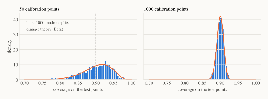
Two things stand out:
- The average is 90% in both panels (90.2% and 90.0%). The guarantee holds.
- The spread depends on . With 50 calibration points, 90% of the runs land between 82.6% and 95.8%, and 11.5% of them fall below 85%. With 1000 points the range shrinks to 88.4%–91.6%.
The orange curve is the theoretical answer, and it matches the bars. For a fixed calibration set, coverage follows a Beta distribution, , whose spread shrinks roughly like . A practical rule of thumb: use at least a few hundred calibration points (1000 is comfortable) if you want each deployed model to land close to 90%.
The simulation loop takes ten lines, reusing model and the splits from above:
scores_all = np.abs(np.r_[y_cal, y_te] - model.predict(np.r_[X_cal, X_te]))
rng = np.random.default_rng(1)
n, covs = 50, []
for _ in range(1000):
    idx = rng.permutation(len(scores_all))
    cal, test = scores_all[idx[:n]], scores_all[idx[n:]]
    k = int(np.ceil((n + 1) * (1 - alpha)))
    covs.append(np.mean(test <= np.sort(cal)[k - 1]))
print(f"mean {np.mean(covs):.3f}, 5-95%: {np.percentile(covs, 5):.3f}-{np.percentile(covs, 95):.3f}")
# mean 0.902, 5-95%: 0.826-0.958
5. What split conformal costs you#
Split conformal is simple and works with any model, but it has two costs that motivate the rest of the series:
- One width for everyone. Every house gets ± $71,800, whether it's an ordinary home where the model is precise or a rare mansion where it is guessing. Part 2 fixes this by changing the score.
- It spends data on calibration. A quarter of the dataset never trains the model. With 20,000 points that's fine. With 40, it hurts. Part 4 shows how to avoid the split.
Recap#
- Split conformal: train on one part, compute scores on a calibration part, take = the -th smallest score, and predict .
- Why it works: with exchangeable data, the new score is equally likely to take any of the ranks, so it is below the -th smallest with probability .
- The accounts for the new point. It matters for small calibration sets.
- Coverage is an average over calibration sets and new points. A single calibration set gives coverage that varies around 90%, by less as grows.
- On California house prices, a model we treated as a black box got intervals with 89.5% test coverage.
Next up — Part 2: Intervals That Adapt. A band of ± $71,800 for every house is honest on average, but it is too wide for easy houses and too narrow for hard ones. We'll see how badly, and fix it by changing the score.