
Conformal Prediction, Step by Step — Part 4: Full Conformal and the Middle Ground
November 7, 2026 · 8 min read · Conformal Prediction, Uncertainty Quantification, Machine Learning, Statistics
This is the most theoretical part of the series. Parts 5 and 6 don't depend on it, so feel free to skip ahead and come back later.
Every method so far used split conformal: train the model on one part of the data, calibrate on another. With 20,000 houses that is no problem. But imagine you have 40 patients, or 30 expensive lab experiments. Giving half of them to calibration means the model learns from only 20 or 15, and a weaker model means wider intervals.
This post answers the question "what does splitting cost us, and can we avoid it?" This time the recipe changes how calibration is done:
| Step | Split conformal (Parts 1–3) | This post |
|---|---|---|
| 1. Score | on a separate calibration set | on every point, using models that treat the new point like the others |
| 2. Quantile | from calibration scores | same rank idea, with scores |
| 3. Keep | answers with score | same |
1. Full conformal: let the new point join the class#
Full conformal prediction (also called transductive) is the original form of the method, from Vladimir Vovk and colleagues around 2000. Split conformal came later as a cheaper shortcut.
The idea answers one question about each possible answer for a new input : if the true answer were , would the new point look like an outsider?
To check one candidate :
- Add the pair to the training points, giving points.
- Refit the model on all points.
- Score every point with this model: for the old points and for the new one.
- Rank the new point's score among all scores. Its conformal p-value is the share of scores that are at least as large:
Keep if . The prediction set is every that passes:
ELI5: a new student joins a class, and we want to guess their height. For each guess, we let the student join the class photo at that height and ask: does this student stick out? A guess of 1.70 m in a class of 12-year-olds sticks out badly, so we drop it. A guess of 1.50 m blends in, so we keep it. The heights that blend in form the interval.
Why it's valid. If is the true answer, then the model was fitted to exchangeable points and treats all of them the same way. So the scores are exchangeable, and the new score is equally likely to take any rank. That's exactly the rank argument from Part 1: the true answer gets a p-value at or below with probability at most , so it is kept with probability at least .
Notice the residuals are measured on points the model was trained on. In Part 0 that was a mistake, because training errors are too small. Here it's fine, because the new point is in the training set too. All points get the same "home advantage", so the comparison is fair.
Here is the p-value for every candidate answer, using ridge regression on 30 points, at a new input :
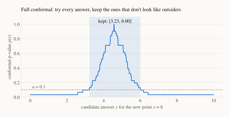
Near the model's prediction, the new point blends in and the p-value is high. Far away, the new point is the worst-fitting of all 31, so its p-value drops to (it is always at least as large as itself). The interval is the region above the orange line: .
The code is a direct translation of the four steps. It's slow (one refit per candidate), but it shows the method plainly:
import numpy as np
from sklearn.linear_model import Ridge

rng = np.random.default_rng(4)
x = rng.uniform(0, 10, 30)
y = 1 + 0.6 * x + rng.normal(0, 1, 30)
x_new, alpha = 6.0, 0.1

X_aug = np.append(x, x_new).reshape(-1, 1)
kept = []
for cand in np.linspace(0, 10, 1001):                     # every candidate answer
    y_aug = np.append(y, cand)                            # 1. add the new point
    model = Ridge(alpha=1.0).fit(X_aug, y_aug)            # 2. refit on all n + 1
    r = np.abs(y_aug - model.predict(X_aug))              # 3. score all n + 1
    if np.mean(r >= r[-1]) > alpha:                       # 4. keep if p-value > alpha
        kept.append(cand)
print(f"interval: [{min(kept):.2f}, {max(kept):.2f}]")
# interval: [3.23, 6.00]
2. The cost: a refit for every candidate answer#
Full conformal uses every point for both training and calibration, so no data is wasted. The price is computation. For each new input we refit the model once per candidate answer. With a grid of 1,000 candidates and 1,000 new inputs, that is a million refits. For a neural network, that's out of the question. For classification it's cheaper (one refit per class), but still one full set of refits per test input.
There are exact shortcuts for a few models. For ridge regression, the residuals turn out to be linear in the candidate , so the whole p-value curve can be computed in one pass without a grid (Nouretdinov, Melluish and Vovk, 2001). Similar tricks exist for the lasso and for nearest neighbours. For most models, though, there is no shortcut.
That's why split conformal took over in practice: one fit, no matter how many new inputs. It pays by giving up some data.
3. The middle ground: jackknife+ and CV+#
Is there something between "one fit, half the data" and "millions of fits, all the data"? Yes, and the most popular choice comes from Barber, Candès, Ramdas and Tibshirani (2021).
Jackknife+ uses leave-one-out models. For each training point , fit a model on all points except , and record its error on the point it left out:
Each is an honest held-out error, and every point gets one. For a new input , each leave-one-out model makes its own prediction , and the interval combines them:
Here means the -th smallest of the values, and means the -th smallest. In words: each leave-one-out model proposes a range "my prediction ± my held-out error", and the interval spans from a low quantile of the lower ends to a high quantile of the upper ends.
The "+" matters. The plain jackknife uses the full model's prediction a quantile of the , and it can badly under-cover when the model is unstable. Using each fixes that.
CV+ does the same thing with folds instead of leave-one-out models. Fit models, each leaving out one fold, and use each point's error from the model that didn't see it. With , that's 10 fits instead of .
The guarantee is a little weaker. In the worst case, jackknife+ guarantees (80% when you ask for 90%), and CV+ slightly less. In practice, coverage is almost always close to , as the table below shows.
from sklearn.linear_model import Ridge

def jackknife_plus(X, y, X_new, alpha=0.1, make_model=lambda: Ridge(alpha=1.0)):
    n = len(y)
    lo, hi = [], []
    for i in range(n):                                    # n leave-one-out models
        keep = np.arange(n) != i
        m = make_model().fit(X[keep], y[keep])
        r_i = abs(y[i] - m.predict(X[i:i + 1])[0])        # held-out error on point i
        mu = m.predict(X_new)
        lo.append(mu - r_i)
        hi.append(mu + r_i)
    lo, hi = np.sort(lo, axis=0), np.sort(hi, axis=0)
    k_lo = int(np.floor(alpha * (n + 1)))
    k_hi = int(np.ceil((1 - alpha) * (n + 1)))
    return lo[k_lo - 1], hi[k_hi - 1]

# 50 points with 10 features
rng = np.random.default_rng(0)
beta = np.linspace(1, -1, 10)
X = rng.normal(size=(50, 10)); y = X @ beta + rng.normal(size=50)
X_te = rng.normal(size=(2000, 10)); y_te = X_te @ beta + rng.normal(size=2000)
lower, upper = jackknife_plus(X, y, X_te)
print(f"coverage {np.mean((y_te >= lower) & (y_te <= upper)):.3f}, width {np.mean(upper - lower):.2f}")
# coverage 0.923, width 3.73
4. How much does splitting cost?#
To compare the four methods fairly, we use a simple setting where we know the truth: 10 features, a linear signal, Gaussian noise with standard deviation 1, and ridge regression as the model. If we knew the true line, the best 90% interval would have width . We vary the number of labelled points and average over 100 datasets:
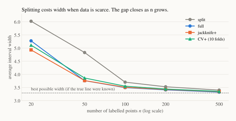
| Method | Fits needed | |||||
|---|---|---|---|---|---|---|
| Split | 1 | 6.02 (91%) | 4.83 (93%) | 3.70 (90%) | 3.53 (91%) | 3.40 (91%) |
| Full | 1 per candidate, per new input | 5.27 (91%) | 3.76 (90%) | 3.49 (89%) | 3.41 (91%) | 3.32 (90%) |
| Jackknife+ | 4.93 (91%) | 3.76 (90%) | 3.51 (90%) | 3.43 (91%) | 3.34 (90%) | |
| CV+ (10 folds) | 10 | 5.11 (92%) | 3.86 (90%) | 3.55 (90%) | 3.44 (91%) | 3.35 (90%) |
Each cell is the average width, with coverage in brackets. Three lessons:
- With little data, splitting hurts a lot. At , split conformal's intervals are about 28% wider (4.83 against 3.76). Its model learned 10 coefficients from only 25 points.
- With plenty of data, it barely matters. At , the four methods are within 3% of each other and close to the best possible 3.29.
- Every method kept about 90% coverage, including jackknife+ and CV+, despite their weaker worst-case guarantee.
5. Which one should I use?#
| Situation | Use | Why |
|---|---|---|
| Thousands of points, or an expensive model (deep nets, big boosted ensembles) | Split | One fit. With lots of data, splitting costs almost nothing. |
| Small data (tens to a few hundred points), model cheap enough to fit 5–20 times | CV+ | Most of full conformal's efficiency for fits. |
| Small data and a very cheap model | Jackknife+ | Slightly tighter than CV+, but needs fits. |
| A model with an exact shortcut (ridge, lasso, k-NN), or a theory paper | Full | Exact guarantee and no wasted data. |
In code you rarely write these by hand. MAPIE, the main Python library, offers SplitConformalRegressor, CrossConformalRegressor (jackknife+ and CV+) and JackknifeAfterBootstrapRegressor, a cheaper relative of jackknife+ that reuses bagged models instead of refitting.
Recap#
- Full (transductive) conformal: for each candidate answer, add it to the data, refit, and keep it if the new point doesn't stand out among the scores. No data is wasted and the guarantee is exact, but it needs one refit per candidate per new input.
- Split (inductive) conformal is the cheap shortcut: one fit, at the cost of setting aside calibration data.
- Jackknife+ ( fits) and CV+ ( fits) are the middle ground. They use every point for both jobs, with a worst-case guarantee of that is close to in practice.
- Splitting costs a lot with tens of points and almost nothing with thousands.
Next up — Part 5: When Exchangeability Breaks. Every guarantee so far rests on one assumption: new data looks like the old data. In real deployments, it often doesn't. The customers change, or the world drifts over time. We'll see coverage fall from 90% to 70%, and two ways to win it back.