
Conformal Prediction, Step by Step — Part 5: When Exchangeability Breaks
November 7, 2026 · 7 min read · Conformal Prediction, Uncertainty Quantification, Machine Learning, Time Series
Every guarantee in this series so far has rested on one assumption, stated back in Part 0: exchangeability. The new point must come from the same source as the calibration points, so that it could have been any one of them.
Real deployments break this all the time. A credit model built on last year's applicants meets this year's. A medical model calibrated in one hospital is used in another. A sales forecast meets a market that keeps growing. This post shows how badly coverage suffers when the assumption fails, and two ways to win it back. This time the recipe changes the weights: not every calibration point counts equally any more.
| Step | Parts 1–4 | This post |
|---|---|---|
| 1. Score | as before | as before |
| 2. Quantile | every calibration score counts equally | scores are weighted: by similarity to the new point, or by time |
| 3. Keep | answers with score | same |
1. What exchangeability really says#
Formally, the points (each ) are exchangeable if shuffling them doesn't change their joint distribution. Every ordering is equally likely. That's the precise version of "the new point could have been any of the calibration points," and it's exactly what the rank argument in Part 1 needed: the new score is equally likely to land in any of the slots.
Two common ways it fails:
- Covariate shift. The inputs change, but the relationship between inputs and outputs doesn't. A house-price model calibrated on suburban homes is used in a city centre. The same features mean the same prices, but now we see different features.
- Drift over time. The world itself changes. Data that arrives in order (a time series) is almost never exchangeable: next month isn't a random draw from the past, it comes after it.
2. Covariate shift: weighted conformal prediction#
Let's go back to the toy data from Parts 0–2, where the noise grows to the right. This time the training and calibration inputs are centred on , but the test inputs move to , where the noise is larger:
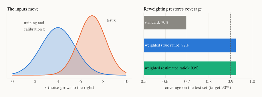
Standard split conformal, calibrated where the noise is small, covers only 70% of test points, averaged over 200 repetitions. Its was learned on mostly easy points and is too small for the harder region where the test points live.
The fix: count the calibration points that look like test points more. Weighted conformal prediction (Tibshirani, Barber, Candès and Ramdas, 2019) gives each calibration point a weight
the ratio of how common is at test time to how common it was in calibration. Points from regions that are rare in calibration but common at test time get large weights. Step 2 then takes a weighted quantile: for a new input , normalize the weights,
and let be the smallest score such that the calibration weights at or below it add up to at least :
The new point's own weight is treated as if it sits at a score of . That's the weighted version of the "" from Part 1. If the weights below every score never reach , , an honest "I can't promise this." With all weights equal, this is exactly ordinary split conformal.
ELI5: this is how polls work. If a survey reached too many retirees and too few students, pollsters don't throw it away. They count each student's answer a bit more, so the sample looks like the population they care about.
But we don't know . We usually don't need to, as long as we have unlabelled test inputs. That's often realistic: you know which houses you'll be asked to price before you know their prices. Train a classifier to tell calibration inputs from test inputs. If it outputs , then with equal sample sizes
With estimated weights, coverage is 92%, just as good as with the true ones.
import numpy as np
from sklearn.linear_model import LogisticRegression

def weighted_quantile(s_cal, w_cal, w_new, alpha=0.1):
    order = np.argsort(s_cal)
    s, w = s_cal[order], w_cal[order]
    cum = np.cumsum(w) / (w.sum() + w_new[:, None])        # one row per new input
    ok = cum >= 1 - alpha
    return np.where(ok.any(axis=1), s[ok.argmax(axis=1)], np.inf)

# x_cal, s_cal: calibration inputs and scores; x_test: unlabelled test inputs
feats = lambda x: np.column_stack([x, x ** 2])
clf = LogisticRegression().fit(feats(np.r_[x_cal, x_test]),
                               np.r_[np.zeros(len(x_cal)), np.ones(len(x_test))])
odds = lambda x: (p := clf.predict_proba(feats(x))[:, 1]) / (1 - p)
q_hat = weighted_quantile(s_cal, odds(x_cal), odds(x_test))   # one threshold per test input
Two warnings. First, the guarantee assumes that only the inputs moved. If the relationship between and also changed (the same house is now worth more), reweighting can't detect it. Second, reweighting costs data. Here, only a small fraction of the 500 calibration points come from the test region, and the weights make the effective sample size about 29 points. That's why coverage varies more between repetitions (83% to 99% for the middle 90% of runs). If the test region has no calibration points at all, no method can help: you can't calibrate on data you've never seen.
3. Time series: when the past keeps moving#
Now the harder case. In the Time Series, Era by Era series we forecast monthly airline passengers from 1949 to 1960. The simplest sensible forecast there was the seasonal naive: next month will be the same as the same month last year. Let's put conformal intervals around it.
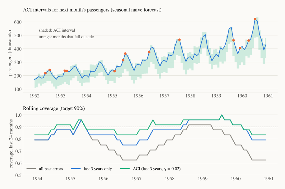
We do it online, as we would in real use. Each month, we take the absolute errors of all past forecasts, build an interval for next month from them, then see the real value and record the new error. We start in 1952, once two years of errors exist, which gives 108 forecast months.
The trouble is that this series grows and its seasonal swings grow with it, so errors from 1950 are much smaller than errors from 1958. Errors from the past are not exchangeable with errors from the future. Here are three ways to build the interval:
| How the interval is built | Coverage 1952–1960 | Coverage in the last 4 years |
|---|---|---|
| All past errors (plain split conformal) | 76.9% | 77.1% |
| Only the last 3 years of errors | 84.3% | 87.5% |
| ACI on the last 3 years | 88.0% | 89.6% |
All past errors (grey) gets worse as the series grows: the old, small errors keep pulling the interval too tight. Its 24-month coverage falls to 63% by 1960.
A sliding window (blue) forgets old errors and does better. But it reacts slowly, and three years is still a long memory for a series that grows this fast.
Adaptive conformal inference (ACI; Gibbs and Candès, 2021) adds a feedback loop. Instead of a fixed , it keeps a running level and nudges it after every step:
After a miss, drops by , so the next interval is built from a higher quantile and is wider. After a hit, rises by , so the interval tightens a little. Because a miss moves nine times more than a hit, the two balance out exactly when misses happen 10% of the time.
ELI5: a thermostat. If the room is too cold, it turns the heat up; if it's too warm, it turns it down. It doesn't need to know why the temperature is changing, only whether it's above or below the target.
ACI's guarantee is different, and remarkable. It holds for any sequence of data, even one chosen by an adversary, with no exchangeability at all. Over steps, the share of misses is close to :
The price: it's a promise about the long-run average, not about each step. ACI can miss several months in a row and then make up for it with extra-wide intervals. And with only 108 months here, the bound is loose: . In practice ACI did much better than its bound (88% coverage), but short series are hard for any online method.
Choosing . A larger reacts faster but makes intervals jumpier. If drops to 0 or below, the interval becomes infinite. We used , which never needed an infinite interval on this series. Newer methods such as conformal PID control (Angelopoulos, Candès and Tibshirani, 2023) add more "controller" terms that help with trends.
import numpy as np
import statsmodels.api as sm

y = sm.datasets.get_rdataset("AirPassengers").data["value"].to_numpy(dtype=float)
scores = np.abs(y[12:] - y[:-12])               # seasonal-naive errors, one per month

alpha, gamma, window = 0.1, 0.02, 36
a_t, misses = alpha, []
for t in range(24, len(scores)):                 # start once 2 years of errors exist
    past = scores[max(0, t - window):t]
    k = int(np.ceil((len(past) + 1) * (1 - a_t)))
    q = np.inf if a_t <= 0 or k > len(past) else np.sort(past)[k - 1]
    err = float(scores[t] > q)                   # did this month fall outside?
    misses.append(err)
    a_t += gamma * (alpha - err)                 # the ACI update
print(f"coverage: {1 - np.mean(misses):.3f} over {len(misses)} months")
# coverage: 0.880 over 108 months
Wouldn't a better score help? Partly. Part 2's lesson applies here too: the errors grow with the level, so a relative error is a more natural score. But it doesn't remove the drift, it just changes its direction. On this series, relative errors happen to shrink over the years, and plain conformal with the relative score over-covers at 99%. ACI corrects in either direction, so it works with any score.
Recap#
- Conformal guarantees need exchangeability. When test data looks different from calibration data, coverage can fall a long way: 70% instead of 90% under a simple input shift, 77% on a growing time series.
- Covariate shift: weight calibration points by and take a weighted quantile. The weights can be estimated with a classifier using unlabelled test inputs. This restored 92% coverage. It assumes only the inputs moved, and it costs effective sample size.
- Time series: a sliding window helps a bit. ACI adds a feedback loop on that guarantees the long-run miss rate approaches for any data sequence. On AirPassengers it lifted coverage from 77% to 88%.
- No method can calibrate for situations it has never seen.
Next up — Part 6: Conformal Prediction for LLMs, and a Checklist. Large language models state their confidence freely and are often overconfident. We use conformal ideas to decide when an LLM should answer and when it should say "I'm not sure", with a guarantee on how often it's wrong. The series ends with a practical checklist.