
Conformal Prediction, Step by Step — Part 3: Prediction Sets for Classification
November 7, 2026 · 7 min read · Conformal Prediction, Uncertainty Quantification, Machine Learning, Statistics
So far every model predicted a number, and conformal prediction put an interval around it. Most models in practice are classifiers: they predict a label. What is the "interval" for a label?
It is a set. Instead of answering "this digit is a 4," the model answers "this digit is in ," and we guarantee that the true label is in the set 95% of the time. When the input is clear, the set has one label. When it is unclear, the set grows. The size of the set becomes an honest, easy-to-read measure of uncertainty.
The recipe is still the same. This time we change step 1 (the score) and step 3 (the output):
| Step | Regression (Parts 1–2) | Classification (this post) |
|---|---|---|
| 1. Score | how far is from the prediction | how unlikely the model thinks the true label is |
| 2. Quantile | from calibration scores | same |
| 3. Keep | an interval of numbers | a set of labels |
1. The setup: handwritten digits#
We use scikit-learn's digits dataset: 1,797 tiny 8×8 images of handwritten digits 0–9. A logistic regression trained on just 300 of them gets 93.5% accuracy on the rest. That's good, but it means about one digit in fifteen is labelled wrongly, and the model doesn't tell us which ones.
The model outputs a probability for each class, , and the 10 probabilities sum to 1. We keep the remaining 1,497 images and split them into 750 for calibration and 747 for testing.
Which coverage level? Our model is right 93.5% of the time just by predicting its top label, so a 90% set is too easy a target: it can be met by sometimes returning an empty set, which isn't useful. (With 90% sets, about 6% of the sets come out empty.) A useful rule: pick a coverage level above the model's accuracy. We'll ask for 95% ().
2. The simple method: keep every label that's likely enough#
The most natural score is one minus the probability the model gives the true label:
If the model is confident and right, the score is near 0. If it gave the true label little probability, the score is near 1. Step 2 is unchanged: is the -th smallest calibration score. Step 3 keeps every label whose score is at most :
In words: keep every label with probability above a calibrated threshold. This is called LAC (for least ambiguous set-valued classifier; it gives the smallest sets on average). The guarantee is the same as in Part 1, by the same rank argument.
Here is what the sets look like:
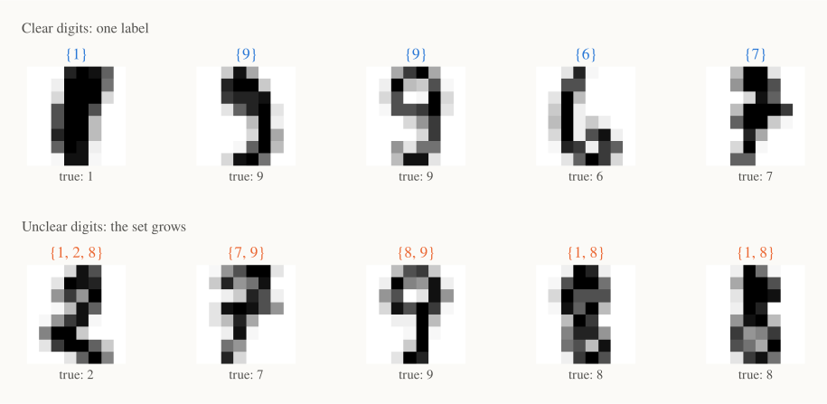
The top row gets single labels. The bottom row gets sets: a 7 that looks a bit like a 9 gets , and an 8 with a thin middle gets . The true label is always in the set here, and that is no accident: it happens 95% of the time on average.
ELI5: a doctor who isn't sure says "it's either flu or a cold," not "it's flu." That is more useful, because the doctor knows what to rule out next, and so does the patient.
3. In code: LAC#
import numpy as np
from sklearn.datasets import load_digits
from sklearn.linear_model import LogisticRegression
from sklearn.model_selection import train_test_split

X, y = load_digits(return_X_y=True)
X_tr, X_rest, y_tr, y_rest = train_test_split(X / 16, y, train_size=300,
                                              random_state=0, stratify=y)
model = LogisticRegression(max_iter=2000).fit(X_tr, y_tr)

idx = np.random.default_rng(0).permutation(len(y_rest))
cal, te = idx[:750], idx[750:]
p_cal = model.predict_proba(X_rest[cal])
p_te = model.predict_proba(X_rest[te])

alpha = 0.05
scores = 1 - p_cal[np.arange(len(cal)), y_rest[cal]]     # 1. score
k = int(np.ceil((len(scores) + 1) * (1 - alpha)))
q_hat = np.sort(scores)[k - 1]                           # 2. quantile
sets = p_te >= 1 - q_hat                                 # 3. keep: one row of True/False per image

covered = sets[np.arange(len(te)), y_rest[te]]
print(f"threshold {1 - q_hat:.3f}, coverage {covered.mean():.3f}, "
      f"average set size {sets.sum(1).mean():.2f}")
# threshold 0.272, coverage 0.948, average set size 1.06
A label goes into the set if the model gives it at least 27% probability. On average, sets have 1.06 labels: almost always one, occasionally two.
4. The catch: LAC short-changes hard inputs#
LAC has the same weakness as Part 1's constant-width band. It promises 95% on average, and it meets that promise mostly on easy inputs. To see this, group the test digits by how confident the model is (its top probability), and measure coverage in each group. The numbers below are averaged over 50 random calibration/test splits:
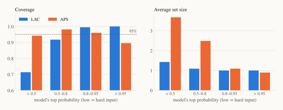
Look at the blue bars on the left. On inputs where the model's top probability is below 0.5 (about 10% of digits), LAC covers only 71%, far below 95%. It makes up for it by covering almost 100% of the easy inputs. The right panel shows why: LAC's sets barely grow on hard inputs (1.4 labels on average).
The reason is in the score. LAC asks "is this label's probability above 27%?" On a hard input the model spreads its probability over many labels, so the true label often gets less than 27%, even when it is the second or third most likely.
5. Adaptive sets: APS#
Adaptive prediction sets (APS; Romano, Sesia and Candès, 2020) change the question. Instead of "is this label likely enough?", ask "how much probability do I have to collect before I reach this label?"
Sort the labels from most to least likely, and add up their probabilities in that order. The score of the true label is the running total at the point where you reach it:
The first term is the probability of all labels ranked above . The second adds a random fraction of 's own probability (more on that below). The set is then built the same way: walk down the sorted labels and keep adding them while the running total is at most .
Why this adapts: on a confident input, the top label alone has probability 0.99, so the running total jumps past immediately and the set has one label. On an unclear input, the probability is spread out, the total grows slowly, and the set takes in several labels before passing .
The orange bars show the effect. APS covers 94% of the hardest inputs, and between 90% and 98% in every group. It pays for this with bigger sets where they are needed: 3.7 labels on the hardest inputs, about 1 on the easy ones. The average set size is 1.66 against LAC's 1.06.
About the random . Scores built from probabilities have many near-ties, and without the coin flip APS would over-cover (give more than 95%, with bigger sets than needed). The randomization makes coverage land on 95% exactly. It has one odd side effect: on very confident inputs, the coin flip sometimes drops even the top label, giving an empty set (3.7% of sets here). That's why APS covers "only" 90% of the most confident group. Libraries usually offer an option to always keep the top label, which removes empty sets at the price of a little extra coverage.
RAPS (regularized APS; Angelopoulos et al., 2021) adds a small penalty for each extra label beyond the first few, which trims long tails of unlikely labels. With a penalty of 0.02 per label, the average set size drops from 1.66 to 1.52 with coverage still at 95%. That makes the most difference with many classes (on ImageNet's 1,000 classes, APS sets can get long).
| Method | Coverage | Avg. set size | Coverage on hardest 10% | Empty sets |
|---|---|---|---|---|
| LAC | 94.9% | 1.06 | 71% | 0.4% |
| APS | 95.0% | 1.66 | 94% | 3.7% |
| RAPS | 95.1% | 1.52 | 92% | 3.4% |
There's no single winner. LAC gives the smallest sets and is the simplest to explain. APS and RAPS treat hard inputs more fairly. If the hard cases are the ones you care about (a doctor triaging unclear scans, say), use APS or RAPS.
6. Coverage for every class#
The same "average hides failures" problem appears across classes. Some digits are just harder to write clearly. Here is LAC's coverage for each true digit:
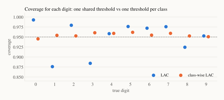
LAC (blue) covers 99% of zeros but only 88% of ones and threes. If a 1 is the class you care most about, the 95% promise doesn't apply to it.
The fix is the Mondrian trick from Part 2: calibrate each class separately. For class , compute from only the calibration images whose true label is , and keep label in a new set if . Each class now has its own guarantee, and in the figure (orange) all ten digits land between 94.5% and 96%. The cost is slightly bigger sets (1.21 labels on average) and the need for enough calibration images of every class: here about 75 per class.
q_class = np.empty(10)
for j in range(10):
    s_j = scores[y_rest[cal] == j]                      # calibration scores for class j only
    k_j = int(np.ceil((len(s_j) + 1) * (1 - alpha)))
    q_class[j] = np.sort(s_j)[k_j - 1]
sets_cw = p_te >= 1 - q_class                           # label j uses its own threshold
covered = sets_cw[np.arange(len(te)), y_rest[te]]
print([round(float(covered[y_rest[te] == j].mean()), 2) for j in range(10)])
One split has only about 75 test images per digit, so its per-class numbers are noisier than the 50-split averages in the figure. The guarantee is about the average over splits, as in Part 1.
Recap#
- For classifiers, conformal prediction returns a set of labels that contains the true label with the chosen probability. The set size is an honest measure of uncertainty.
- Pick a coverage level above the model's accuracy, or you'll get empty sets.
- LAC: score , keep labels with . Smallest sets, simple, but under-covers hard inputs (71% instead of 95% here).
- APS: score = probability mass collected before reaching the true label. Sets grow on unclear inputs, and coverage is much more even (94% on the hardest inputs). RAPS trims the sets with a small penalty.
- Class-wise (Mondrian) calibration gives every class its own guarantee, at the cost of slightly larger sets.
Next up — Part 4: Full Conformal and the Middle Ground. Every method so far set aside a calibration set that the model never learns from. That is fine with thousands of points, but wasteful with fifty. We meet the original, "full" form of conformal prediction, which uses every point for both jobs, and two practical compromises: jackknife+ and CV+. It's the most theoretical part of the series, and Parts 5 and 6 don't depend on it.