
Conformal Prediction, Step by Step — Part 2: Intervals That Adapt
November 7, 2026 · 7 min read · Conformal Prediction, Uncertainty Quantification, Machine Learning, Statistics
Part 1 gave every California house the same interval: prediction ± $71,800. Overall, 89.5% of test houses landed inside, just as promised. But think about what that interval means for two different houses. For an ordinary three-bedroom home in a typical suburb, the model is quite precise, and ± $71,800 is far too cautious. For a rare luxury home, the model is guessing, and ± $71,800 is far too tight.
This post fixes that. The fix keeps the recipe from Part 1 and changes only step 1, the score:
| Step | Part 1 | This post |
|---|---|---|
| 1. Score | an error measured relative to how hard is | |
| 2. Quantile | = the -th smallest score | same |
| 3. Keep | answers with score | same |
Because steps 2 and 3 don't change, the coverage guarantee from Part 1 carries over for free.
1. The problem: honest on average, wrong almost everywhere#
Let's look closer at the toy data from Parts 0 and 1, where the noise grows from left to right. The left panel below is Part 1's constant-width band:
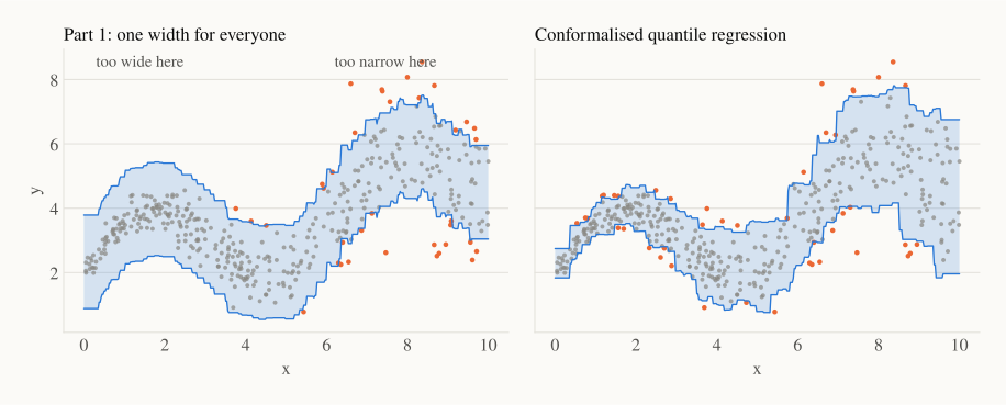
On the left side, the band is much wider than the data needs. On the right side, many points spill out (orange). The 90% average hides two different failures, which we can measure by splitting the test points into five regions of :
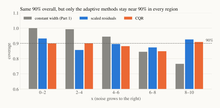
The grey bars are Part 1's band. It covers 100% of points in the quiet region and only 77% in the noisiest one. The average works out to 91%, so the guarantee is technically kept, but no individual region gets what it was promised.
This is the difference between two kinds of coverage:
- Marginal coverage (what Part 1 guarantees): . The probability is taken over all inputs together. The 90% is an average over easy and hard cases.
- Conditional coverage (what we'd really like): for every . Every kind of input gets 90%.
ELI5: a teacher promises that "90% of students will pass." She can keep that promise by passing every student in the easy class and failing a third of the hard class. The parents in the hard class would not call that fair.
A hard truth: exact conditional coverage for every single is impossible to guarantee without assumptions, with any method, when is continuous. We can never have enough calibration points at one particular . What we can do is get much closer by choosing a score that knows which inputs are hard. That's the job of this post.
2. Fix 1: scale the error by how hard the input is#
The idea: a $50,000 miss on a house the model finds easy is a big miss. The same miss on a house the model finds hard is ordinary. So we divide each error by a prediction of its typical size:
where is a second model that predicts how large the error usually is at . Steps 2 and 3 are unchanged. Solving for gives
The width is now : wide where errors are usually large, narrow where they are small. And is still chosen on calibration data, so even if is a poor model, coverage is still 90% on average. A bad costs efficiency, never validity.
How to train . Fit it to predict , but use errors measured on data that the mean model did not train on. This is Part 0's lesson again: training-set errors are too small. In our code, we fit one mean model on the first half of the training data and train on its errors on the second half.
3. Fix 2: conformalized quantile regression (CQR)#
Instead of predicting the middle and then a spread, we can predict the edges of the interval directly. A quantile regression model learns a chosen quantile of given . Train two of them:
- : the 5% quantile ("only 5% of prices are below this"),
- : the 95% quantile.
The band already adapts to the data. But it comes with no guarantee: the quantile models were trained on the training set, so they're usually too tight on new data (Part 0's lesson, once more).
Conformalized quantile regression (Romano, Patterson and Candès, 2019) fixes the band with one calibrated number. The score asks how far outside the band is the true answer?
If is below the band, the first term is positive and measures the miss. If is above, the second term is. If is inside, both are negative and the score is negative, which says how much room was left. Step 2 gives as usual, and step 3 gives
If the quantile models were too tight, and the band widens on both sides. If they were too loose, and it shrinks. Either way the shape comes from the quantile models and the guarantee comes from conformal calibration.
The right panel of the first figure is CQR. It hugs the data where it's tight and opens up where it's noisy. In the coverage chart, both fixes stay within a few points of 90% in every region (85% to 93%). They are also narrower on average: 2.64 (scaled) and 2.51 (CQR) against 2.91 for the constant band.
4. Back to California houses#
Here are the three methods on the house-price data from Part 1, with the same model and the same splits. To see who gets short-changed, we sort the test houses by the model's predicted price and split them into five equal groups:
| Method | Coverage | Average width | Coverage by predicted price, cheapest fifth → priciest fifth |
|---|---|---|---|
| Constant width (Part 1) | 89.5% | 1.44 | 98.4% · 96.2% · 91.3% · 84.9% · 76.8% |
| Scaled residuals | 89.8% | 1.39 | 91.8% · 91.5% · 90.5% · 88.5% · 86.9% |
| CQR | 90.4% | 1.49 | 92.4% · 90.2% · 90.7% · 89.1% · 89.6% |
Widths are in units of $100,000, so 1.44 means the interval spans $144,000 in total.
All three methods keep the 90% marginal promise. The constant band does it by over-covering cheap houses (98%) and under-covering the most expensive fifth (77%), so almost one in four expensive houses falls outside its interval. CQR stays between 89% and 92% in every group.
Notice the widths. CQR is not narrower on average here (1.49 against 1.44). It moves width from where it isn't needed to where it is. For 80% of houses, its width lies between 0.78 and 2.50 (between $78,000 and $250,000). That is the real gain: a buyer of an ordinary home gets a tight, useful range, and a buyer of a mansion gets a range that is honest about the uncertainty.
5. In code: CQR#
Continuing from Part 1's code (same X_tr, X_cal, X_te, model and alpha):
lo_model = HistGradientBoostingRegressor(loss="quantile", quantile=alpha / 2,
                                         random_state=0).fit(X_tr, y_tr)
hi_model = HistGradientBoostingRegressor(loss="quantile", quantile=1 - alpha / 2,
                                         random_state=0).fit(X_tr, y_tr)

# 1. score: how far outside the [lo, hi] band is the truth?
scores = np.maximum(lo_model.predict(X_cal) - y_cal, y_cal - hi_model.predict(X_cal))
k = int(np.ceil((len(scores) + 1) * (1 - alpha)))
q_hat = np.sort(scores)[k - 1]                      # 2. quantile

lower = lo_model.predict(X_te) - q_hat              # 3. keep
upper = hi_model.predict(X_te) + q_hat
inside = (y_te >= lower) & (y_te <= upper)

pred = model.predict(X_te)
fifth = np.digitize(pred, np.quantile(pred, [0.2, 0.4, 0.6, 0.8]))
print(f"q_hat = {q_hat:.3f}, coverage = {inside.mean():.3f}, width = {np.mean(upper - lower):.2f}")
print("by predicted price:", [round(float(inside[fifth == g].mean()), 3) for g in range(5)])
# q_hat = 0.068, coverage = 0.904, width = 1.49
# by predicted price: [0.924, 0.902, 0.907, 0.891, 0.896]
The quantile models were slightly too tight, so : each edge moves out by about $6,800.
6. Coverage for groups you care about#
Sometimes you don't need coverage for every , only for a few groups that matter: regions, product lines, age bands. Then there is a simple trick with an exact guarantee: calibrate each group separately. Compute one per group from that group's calibration points, and use it for new points in that group. Each group then gets its own 90% guarantee, at the cost of needing enough calibration points in every group. This is called Mondrian conformal prediction, and we'll use it in Part 3 to give every class its own coverage.
Recap#
- Split conformal guarantees marginal coverage: 90% on average over all inputs. A constant-width band can hide large failures on hard inputs (77% for the most expensive houses).
- Conditional coverage (90% for every ) can't be guaranteed exactly, but a better score gets much closer. Steps 2 and 3 don't change, so the marginal guarantee stays.
- Scaled residuals: , giving the interval . Train on held-out errors.
- CQR: , giving . It is a strong default for regression.
- Adaptive methods don't always narrow the average width. They put the width where the uncertainty is.
- For coverage within specific groups, calibrate each group separately (Mondrian).
Next up — Part 3: Prediction Sets for Classification. What is the "interval" for a label? We change the score and the output once more, and get sets of labels that grow when the input is unclear, such as for a messy handwritten digit.