
Time Series, Era by Era — Part 0: Learning to Look Before You Forecast
November 5, 2026 · 6 min read · Time Series, Forecasting, Statistics
Every morning you make a forecast without noticing. "It was cold yesterday, it's winter, so it'll probably be cold today." In one sentence you used the recent past (yesterday), a repeating pattern (winter), and a sense of uncertainty ("probably"). Time series forecasting is the same idea written down carefully enough that a computer can do it.
This series walks through forecasting the way the field grew up, one era at a time. Each era kept what worked before and fixed one thing that didn't:
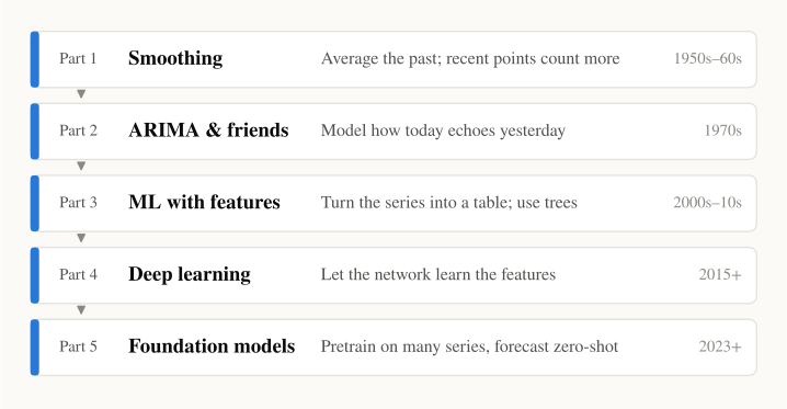
Before any model, though, we need to learn how to look at a time series. This post covers four things every later part relies on:
- what a time series is made of,
- why you can't shuffle it like ordinary data,
- two "dumb" baselines that every model must beat,
- how to score a forecast honestly.
The only background you need is comfort with sums and averages.
1. What is a time series?#
A time series is a list of numbers recorded in order at equal time steps:
Here is the value at time (a day, a month, an hour) and is the most recent time we have observed. A forecast is a guess about a future value:
Read this as "our guess for time , made using data up to time ." The number is the horizon: how many steps ahead we are looking. The hat means "estimate."
What makes this different from ordinary machine learning: order carries information. Shuffle the rows of a house-price dataset and nothing is lost. Shuffle a time series and you destroy the very thing you want to learn.
Throughout the series we'll use one classic dataset: monthly international airline passengers from 1949 to 1960 (Box & Jenkins, 1976).
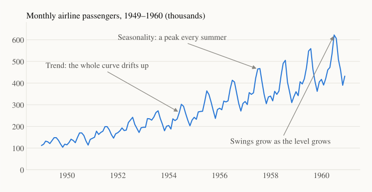
Even without any math, your eye picks up three things.
2. Anatomy: trend, seasonality, noise#
Think of the sea at the beach:
- the tide slowly raises the water level over hours: that's the trend ;
- waves come and go in a regular rhythm: that's seasonality ;
- random splashes you can't predict: that's the residual (noise) .
There are two common ways to put these pieces together.
Additive: the pieces are added up. The seasonal swing has a fixed size, say "+50 passengers every July":
Multiplicative: the pieces are multiplied. The seasonal swing is a fixed percentage, say "+20% every July":
How do you choose? Look at the swings. In our data, the gap between the busiest and quietest month grows from 44 thousand passengers in 1949 to 232 thousand in 1960. The swings grow with the level, so multiplicative fits better. (Taking logs turns a multiplicative series into an additive one, since . You'll see that trick again.)
Pulling the pieces apart#
Classical decomposition separates the components in three steps:
- Trend: average each point with its neighbours over one full year (a centred 12-month moving average). Averaging over a whole cycle cancels the seasonal ups and downs, leaving the slow drift. This is our first taste of smoothing, the topic of Part 1.
- Seasonality: divide the data by the trend, then average the result for each calendar month (all Januaries, all Februaries, …). That gives 12 seasonal factors, scaled so they average to 1.
- Residual: whatever is left, .
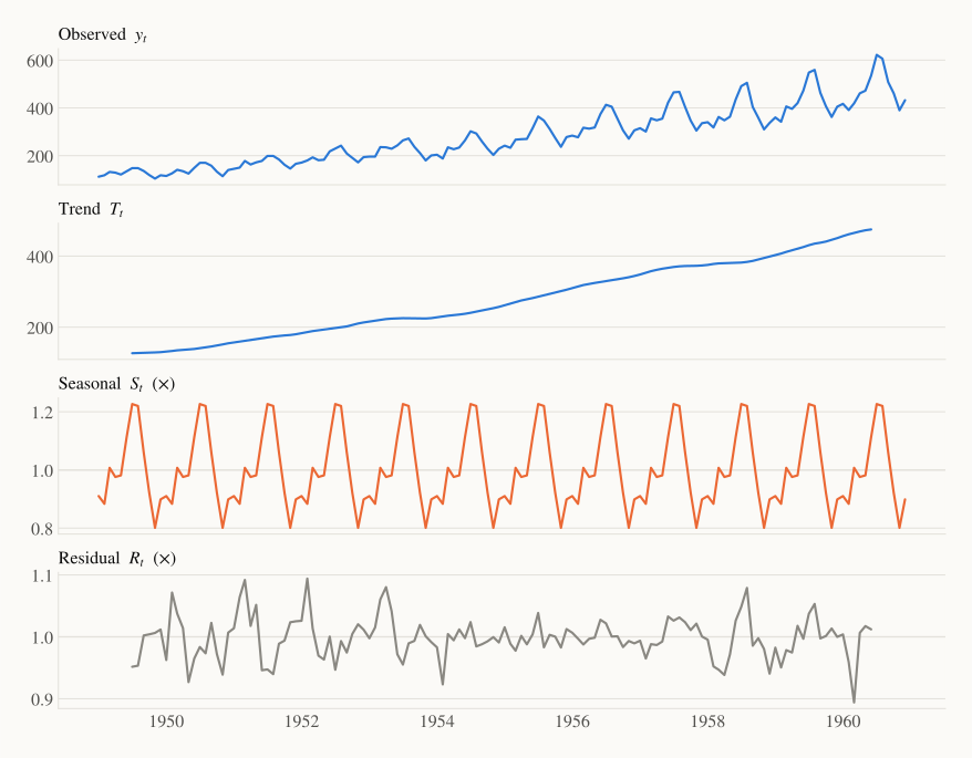
How to read it:
- Trend climbs steadily, roughly quadrupling over 12 years. (It is missing for the first and last 6 months because a centred 12-month window needs 6 months on each side.)
- Seasonal factors peak at 1.23 in July (23% above trend) and bottom out at 0.80 in November (20% below). That's summer holidays.
- Residual hovers around 1 with no obvious pattern. That's what we want: if the residual still had structure, our decomposition would have missed something.
Every method in this series is, at heart, a different way of estimating these components and projecting them forward.
3. Why you can't shuffle: the time split#
In ordinary ML you split data randomly into train and test sets. Do that with a time series and the model trains on, say, March 1960 and is then "tested" on February 1960. It has seen the future.
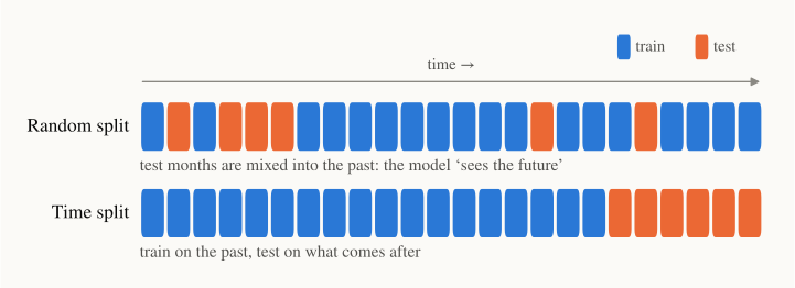
It's like studying with the answer key next to you: great exam score, no real skill. This mistake is called leakage. It quietly makes almost any model look better than it really is.
The rule: train on the past and test on what comes after. For our data, we train on 1949–1958 (120 months) and test on 1959–1960 (24 months).
4. Two baselines every model must beat#
Before building anything clever, build something dumb. A baseline tells you whether the clever thing is actually earning its keep.
Naive forecast: tomorrow will look like today.
Seasonal naive forecast: this July will look like last July.
Here is the season length ( for monthly data) and is the smallest whole number that makes , i.e. "the most recent observed value from the same month." For a 24-month forecast, both 1959 and 1960 simply copy 1958.
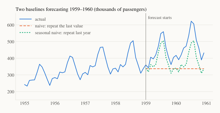
The naive forecast (flat dashed line) ignores the seasons completely. The seasonal naive forecast gets the shape right but sits too low, because it doesn't know the series keeps growing. Fixing exactly that, shape plus growth, is what Holt–Winters smoothing does in Part 1.
5. Scoring a forecast#
Let be the error at each test point, and the number of test points. Four metrics show up everywhere.
MAE (mean absolute error): the average miss, in the data's own units.
RMSE (root mean squared error): like MAE, but squaring punishes big misses more. If RMSE is much larger than MAE, a few bad misses are driving the error.
MAPE (mean absolute percentage error): the average miss as a percentage, so it's easy to explain to a manager. But it blows up when is near zero (think daily sales of a rare product).
MASE (mean absolute scaled error): MAE divided by the MAE of the seasonal naive method on the training data. It has no units, so you can compare it across datasets. Values below 1 mean "better than the typical year-over-year change seen in training."
Here is how our two baselines score on 1959–1960:
| Method | MAE | RMSE | MAPE | MASE |
|---|---|---|---|---|
| Naive | 115.2 | 137.3 | 23.6% | 4.03 |
| Seasonal naive | 71.2 | 77.0 | 15.5% | 2.49 |
Simply knowing about seasons cuts the error by about 40%. These two rows are the bar every later method in this series has to clear.
One test period is not enough: rolling-origin evaluation#
Scoring on a single test window is like judging a student by one exam. Maybe 1959 was unusually easy. Rolling-origin evaluation (also called time-series cross-validation) repeats the exercise: train up to some point, forecast the next few steps, slide the cut-off forward, and repeat. Then average the scores.
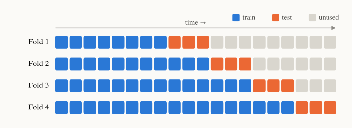
Notice that every fold still respects time: the test block always comes after its training block.
6. In code#
Everything above fits in a few lines of Python (NumPy + statsmodels):
import numpy as np
import statsmodels.api as sm

y = sm.datasets.get_rdataset("AirPassengers").data["value"].to_numpy()
train, test = y[:120], y[120:]            # 1949–1958 | 1959–1960
m = 12                                    # season length

naive = np.full(len(test), train[-1])     # repeat the last value
snaive = np.tile(train[-m:], 2)           # repeat last year, twice

scale = np.mean(np.abs(train[m:] - train[:-m]))
for name, fc in [("naive", naive), ("seasonal naive", snaive)]:
    e = test - fc
    print(f"{name:15s} MAE={np.mean(abs(e)):.1f}  "
          f"RMSE={np.sqrt(np.mean(e**2)):.1f}  "
          f"MAPE={100*np.mean(abs(e/test)):.1f}%  MASE={np.mean(abs(e))/scale:.2f}")
Recap#
- A time series is ordered data; a forecast uses only the past.
- Most series are trend + seasonality + noise, combined additively (fixed-size swings) or multiplicatively (swings that grow with the level).
- Never shuffle. Train on the past, test on the future, ideally over several rolling folds.
- Always compare against naive and seasonal naive. A fancy model that can't beat them isn't worth its complexity.
- Use MAE/RMSE for errors in real units, MAPE for percentages (watch out near zero), MASE for comparisons across series.
Next up — Part 1: Smoothing. The seasonal naive forecast trusted only last year. What if we trusted all the past, but recent data a bit more? That simple idea, a memory that fades, gives us exponential smoothing and, step by step, Holt–Winters, which learns both the growth and the seasons we just saw.