
Time Series, Era by Era — Part 2b: ARIMA in Practice
November 5, 2026 · 7 min read · Time Series, Forecasting, Statistics
In Part 2a we collected three building blocks:
- I (integrated): difference the series until it is stationary;
- AR: today echoes past values;
- MA: today echoes past surprises.
ARIMA snaps them together like Lego. This post builds the model, fits the famous airline model to our running dataset, checks its work, and produces something no earlier part gave us: a forecast with an honest uncertainty band.
1. ARIMA()#
ARIMA() means: difference the series times, then model what's left with AR() and MA() together. Writing for the differenced series (for example when ):
| Letter | Meaning | Typical values |
|---|---|---|
| number of past values (AR order) | 0–3 | |
| number of differences | 0–2 | |
| number of past shocks (MA order) | 0–3 |
To forecast, the model predicts the differenced series step by step and then "un-differences" (adds the changes back up) to return to the original scale.
Adding seasons: SARIMA#
Monthly data also echoes 12 months back. Seasonal ARIMA adds a second, seasonal set of the same three ingredients, operating at lag :
- : the ordinary part, working at lags 1, 2, 3, …
- : the seasonal part, working at lags ( seasonal differences, seasonal AR terms, seasonal MA terms)
- : season length, 12 for monthly data.
2. The Box–Jenkins loop#
Box and Jenkins didn't only propose a model; they proposed a workflow for building one:
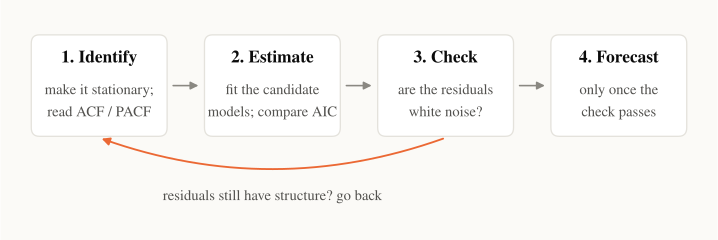
Let's walk the airline data through it.
Step 1: Identify#
From Part 2a we already know the recipe for stationarity: take logs, one ordinary difference (), and one seasonal difference (). Now read the ACF and PACF of the result:
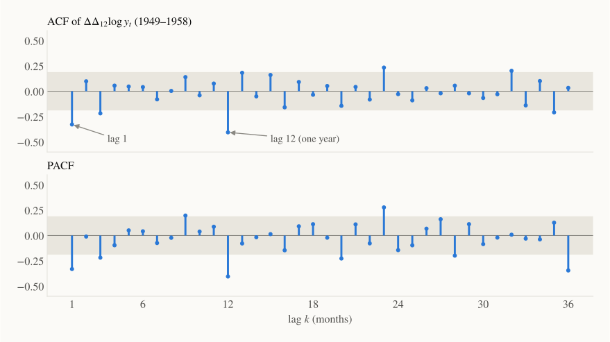
Two sticks clearly stand out in the ACF: lag 1 () and lag 12 (). Everything else stays in, or barely touches, the grey band. Remember the signatures:
- ACF cuts off after lag 1 → an ordinary MA(1) term ();
- ACF cuts off at seasonal lag 12 → a seasonal MA(1) term ().
That gives the candidate SARIMA on . It is so famous that it has its own name, the airline model, because Box and Jenkins built it for exactly this dataset in 1970.
Written out with (log, difference, seasonal difference), it reads:
Just two parameters: (how much last month's surprise carries over) and (how much the surprise from the same month last year carries over). The last term is the interaction between the two: last month's surprise one year ago.
Step 2: Estimate#
The parameters are fitted by maximum likelihood: pick the that make the observed data most probable under the model. On 1949–1958 we get
Both are negative: a surprise tends to be partly undone the next month and the next year. (A busy month is followed by a slightly calmer-than-trend one.)
ACF reading gives a starting point, not a final answer. So we also try a few neighbours and compare them with the Akaike information criterion:
Here is the maximised likelihood (higher means a better fit) and is the number of parameters. The term is a complexity penalty: an extra parameter has to improve the fit enough to pay for itself. Lower AIC is better.
| Model (on ) | AIC |
|---|---|
| — airline | −389.0 |
| −388.6 | |
| −387.3 | |
| −387.2 | |
| −384.8 |
The airline model wins, though not by much. That's typical: several nearby models are often almost equally good.
Step 3: Check#
If the model captured all the echoes, what's left over, the residuals , should look like white noise: no trend, no pattern, no autocorrelation.
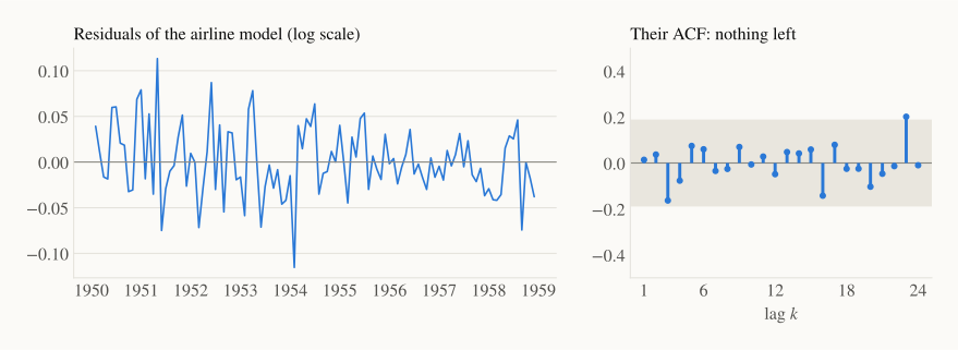
The residuals bounce around zero, and their ACF stays inside the band. The Ljung–Box test turns "stays inside the band" into a single number by combining the first squared autocorrelations of the residuals:
where is the number of residuals and their autocorrelation at lag . Its null hypothesis is "the residuals are white noise." With we get : no evidence of leftover structure. The check passes, so we move on to forecasting. Had it failed, we'd go back to step 1 and try other orders.
Step 4: Forecast, with uncertainty#
Because ARIMA is a full statistical model (it says exactly how the random shocks enter), it also tells us how uncertain each forecast is. Uncertainty grows with the horizon, since each future step adds a new unknown shock.
We fitted the model on , so we forecast on the log scale and back-transform with . Interval endpoints transform directly. One subtlety: of the log-scale forecast gives the median of the forecast distribution, slightly below its mean. For forecasting it's usually the more robust choice anyway.
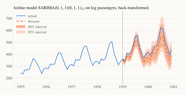
Notice the band widens for 1960 and is wider at the summer peaks, where a 5% surprise means more passengers. All 24 actual months fall inside the 95% interval. The point forecast, however, runs a bit low, especially at the 1960 peak.
3. Results#
Same split as in Parts 0 and 1: train on 1949–1958 and forecast 24 months ahead.
| Method | MAE | RMSE | MAPE | MASE |
|---|---|---|---|---|
| Seasonal naive (Part 0) | 71.2 | 77.0 | 15.5% | 2.49 |
| Holt–Winters, multiplicative (Part 1) | 29.0 | 32.5 | 6.4% | 1.01 |
| Airline model on raw (no log) | 66.4 | 72.0 | 14.4% | 2.32 |
| Airline model on | 39.4 | 43.2 | 8.5% | 1.38 |
| SARIMA on | 36.4 | 40.1 | 7.8% | 1.27 |
Three honest lessons:
- The log matters more than the model. The same airline model goes from MAE 66 to 39 just by working on , because the growing swings break the "constant variance" rule without it.
- Holt–Winters still wins on this test window. Seventy years of practice says neither family dominates; it depends on the series. Unlike Holt–Winters as we used it, though, SARIMA came with calibrated uncertainty bands.
- The best-AIC model isn't the best-test model. has a slightly worse AIC but a better test score. A single 24-month test window is noisy, which is exactly why Part 0 recommended rolling-origin evaluation.
4. A surprise: smoothing is ARIMA#
Here's a neat link back to Part 1. Simple exponential smoothing updates its level by the one-step error :
Take the difference of the second equation and substitute the first:
That is exactly an ARIMA(0,1,1) with . SES and ARIMA(0,1,1) produce the same forecasts. Similarly, Holt's method corresponds to an ARIMA(0,2,2). The "component" view of Part 1 and the "echo" view of Part 2 are two languages for overlapping sets of models. Writing smoothing as a statistical model like this (the ETS framework) is also what gives smoothing methods proper prediction intervals.
5. ARIMAX: letting outside information in#
Plain ARIMA only looks at the series itself. Often you know something else matters: a price change, a holiday, the weather. ARIMAX (regression with ARIMA errors) adds such exogenous variables :
The regression part explains what the outside variables can explain, and the ARIMA part models the echoes in what's left. In statsmodels this is just the exog= argument of SARIMAX.
The catch: to forecast next month, you need for next month. That's fine for calendar features (holidays are known in advance), but harder for something like temperature, which you'd have to forecast first.
6. In code#
import numpy as np
import statsmodels.api as sm
from statsmodels.tsa.statespace.sarimax import SARIMAX
from statsmodels.stats.diagnostic import acorr_ljungbox

y = sm.datasets.get_rdataset("AirPassengers").data["value"].to_numpy()
train, test = y[:120], y[120:]                           # 1949–1958 | 1959–1960

fit = SARIMAX(np.log(train), order=(0, 1, 1), seasonal_order=(0, 1, 1, 12)).fit(disp=False)
fc = fit.get_forecast(24)
mean, ci = np.exp(fc.predicted_mean), np.exp(fc.conf_int(alpha=0.05))

print("theta, Theta:", fit.params[:2].round(2), " AIC:", round(fit.aic, 1))
print("Ljung-Box p:", acorr_ljungbox(fit.resid[13:], lags=[24]).lb_pvalue.iloc[0].round(2))
print("MAE:", np.abs(test - mean).mean().round(1),
      " inside 95% band:", np.mean((test >= ci[:, 0]) & (test <= ci[:, 1])))
theta, Theta: [-0.34 -0.54]  AIC: -389.0
Ljung-Box p: 0.8
MAE: 39.4  inside 95% band: 1.0
(We skip the first 13 residuals because the differencing has nothing to compare against at the start.) If you don't want to pick orders by hand, pmdarima.auto_arima or statsforecast's AutoARIMA search the orders by AIC automatically.
Where ARIMA runs out#
- One series at a time. A retailer with 50,000 products needs 50,000 separately identified and fitted models, and the models can't learn from each other.
- Linear only. Echoes add up linearly; interactions like "promotions work better in December" are out of reach.
- One seasonal period. Like Holt–Winters, SARIMA handles one . Hourly data with daily and weekly cycles needs extensions.
- Exogenous variables are bolted on, and they enter linearly.
Recap#
- ARIMA() = difference times, then AR() + MA(). SARIMA adds a seasonal layer.
- The Box–Jenkins loop: identify (stationarity, ACF/PACF) → estimate (maximum likelihood, compare AIC) → check (residuals are white noise, Ljung–Box) → forecast.
- The airline model SARIMA on log passengers has just two parameters and gives calibrated prediction intervals. On this split it scores MAE 39.4, behind Holt–Winters' 29.0.
- Transform first: the log alone cut the airline model's error by 40%.
- SES is ARIMA(0,1,1) in disguise: components and echoes are two views of the same models.
- ARIMAX adds outside variables, as long as you know their future values.
Next up — Part 3: Machine learning with features. What if we stop writing equations for the echo and instead turn the series into a big table, with lags, rolling averages and calendar columns, and hand it to a gradient-boosted tree? That simple trick lets one model learn from thousands of series at once, and it is how tree models came to dominate forecasting competitions such as M5.