
Time Series, Era by Era — Part 1: Smoothing, a Memory That Fades
November 5, 2026 · 8 min read · Time Series, Forecasting, Statistics
Contents · 8 sections
You run a coffee shop and want to know how many cups to prepare tomorrow. You could:
- copy yesterday: fast to react, but one rainy day throws you off;
- take the average of all past days: calm, but it ignores that your street got busier last month.
Neither feels right. What you actually do in your head is something in between: trust recent days more, but don't forget the older ones completely. That idea, written as a formula, is exponential smoothing. It came out of the 1950s (Brown, Holt, Winters) and, seventy years later, still beats many fancy models on everyday business data.
In this post we build it up in four steps. Each step fixes one weakness of the previous one:
| Step | Method | What it adds |
|---|---|---|
| 1 | Moving average | average the last points |
| 2 | Simple exponential smoothing (SES) | smoothly fading weights instead of a hard cut-off |
| 3 | Holt | a slope, so forecasts can go up or down |
| 4 | Holt–Winters | a seasonal pattern, so forecasts can repeat yearly shapes |
We reuse the notation from Part 0: is the value at time , is the last observed time, and is the forecast steps ahead.
1. Moving average: average the last points#
The simplest smoother takes the average of the last observations and uses it as the forecast:
The window is a dial between two goals:
- small follows the data closely, noise included;
- large irons out the noise, but reacts late when something real changes.
Here is a (made-up) coffee shop that sells about 50 cups a day until a new office opens nearby on day 60:
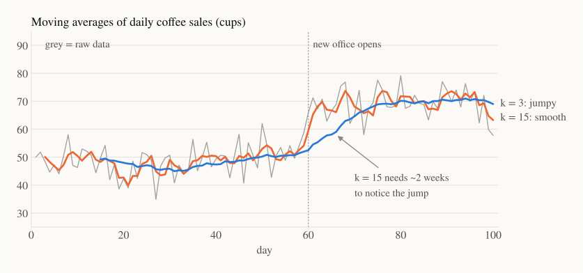
The line is pleasantly calm, but it takes about two weeks to admit that sales have jumped. During those two weeks you'd prepare too little coffee every day.
There's also something odd about the weights. A moving average gives the last points weight each, and everything older weight zero. Is the point from 5 days ago really as important as yesterday's? And is the point from 6 days ago really worth nothing?
2. Simple exponential smoothing: a memory that fades#
The idea in one line#
Keep a running estimate of the "current level" . Each time a new value arrives, nudge the estimate toward it:
Read it as: new estimate = old estimate + α × (how surprised I was). The term is the surprise, i.e. the one-step forecast error. The smoothing parameter decides how big the nudge is.
The forecast is simply the latest level, for every horizon:
Rearranging the update gives the form you'll see in most textbooks, a weighted average of "what I just saw" and "what I believed":
A tiny worked example#
Cups sold over five days, with and the first level set to the first observation ():
| Day | Sold | Forecast | Surprise | New level |
|---|---|---|---|---|
| 1 | 50 | – | – | 50 |
| 2 | 54 | 50 | +4 | 50 + 0.5·4 = 52 |
| 3 | 47 | 52 | −5 | 52 − 0.5·5 = 49.5 |
| 4 | 60 | 49.5 | +10.5 | 49.5 + 0.5·10.5 = 54.75 |
| 5 | 52 | 54.75 | −2.75 | 54.75 − 0.5·2.75 ≈ 53.4 |
So the forecast for day 6 (and for every later day) is about 53 cups. Notice that we only had to remember one number, the current level. That made SES practical on the computers of the 1950s, and it still makes it very fast today.
Why "exponential"?#
Substitute the update into itself again and again:
So SES is also a weighted average of all past observations. The point from steps ago gets weight . These weights shrink geometrically (exponentially), and together with the initial level's weight they add up to exactly 1.
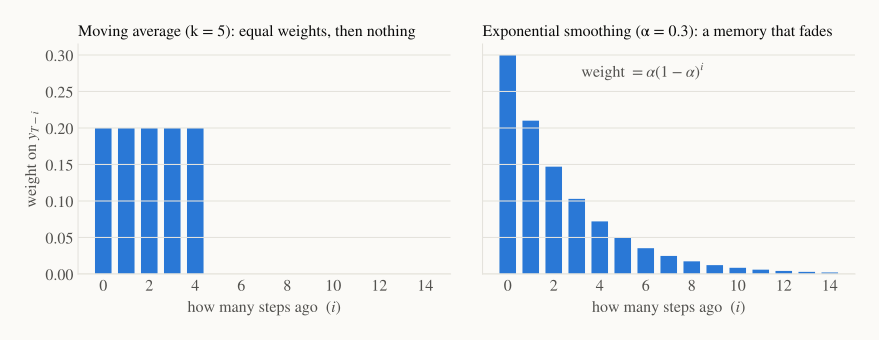
This is the whole difference between the two methods. The moving average has a hard memory: it remembers days perfectly, then forgets completely. Exponential smoothing has a soft memory: yesterday counts most, last week a little, last month almost nothing.
Choosing #
plays the same role as the window :
- close to 1: react fast, trust the newest point. At , SES becomes the naive forecast .
- close to 0: react slowly, average over a long history.
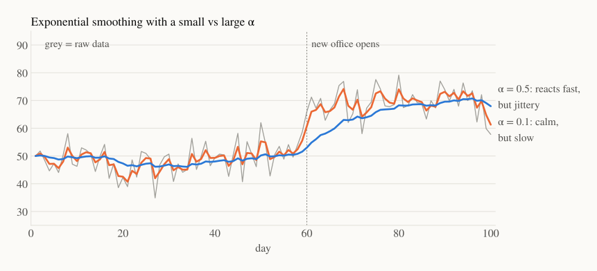
In practice we don't pick by eye. We choose the value that minimises the sum of squared one-step-ahead errors on the training data:
That is, "if I had used this in the past, how wrong would my day-ahead guesses have been?" Libraries do this optimisation for you, usually estimating the starting level at the same time.
3. Holt: add a slope#
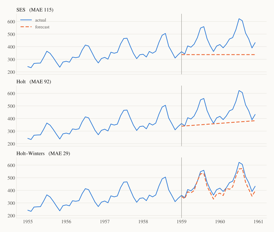
Run SES on the airline passengers from Part 0 and something surprising happens: the optimiser picks . SES turns into the naive forecast, a flat line at the last value. Because the series keeps climbing, "copy the last point" is the best one-step guess a level-only model can make. But a flat line can never follow growth.
Charles Holt's fix (1957) was to track a second quantity: the slope , how much the level changes per step. Both are updated with the same "nudge" logic:
- Level: blend the new observation with where we expected to be, (last level plus one step of slope).
- Slope: blend the latest observed change with the old slope. The new parameter controls how quickly the slope adapts.
The forecast is now a straight line that starts at the last level and continues with the last slope:
ELI5: SES knows where you are. Holt also knows which way you're walking.
One practical warning: straight lines go on forever, and real growth usually doesn't. A popular variant, the damped trend, multiplies the slope by a factor at each future step, so long-horizon forecasts gradually flatten out. It's often the safer default for business data.
4. Holt–Winters: add the seasons#
Holt's line is going up, but it slices straight through the summer peaks and winter dips. Peter Winters (1960) added a third piece: a set of seasonal factors , one per position in the cycle (12 for monthly data). Remember from Part 0 that the airline swings grow with the level, so we use the multiplicative form, where a factor of 1.2 means "20% above the level":
It looks heavy, but each line is the same nudge you already know:
- Level: before using , divide out the seasonal effect (), so a busy July doesn't fool us into thinking the overall level jumped. Here and is the factor for the same month last year.
- Slope: exactly as in Holt.
- Season: compare this month's value with the expected level. If July came in 25% above it, nudge July's factor toward 1.25. The parameter controls how fast the seasonal pattern itself is allowed to change.
The forecast multiplies the trend line by the right month's factor:
(for ; for longer horizons, reuse the most recent factor for that month).
If this reminds you of the decomposition in Part 0, it should: Holt–Winters is a decomposition into level, trend and season that updates itself online, one observation at a time.
5. Results on the airline data#
Same split as Part 0: train on 1949–1958 and forecast all of 1959–1960 in one go.
| Method | MAE | RMSE | MAPE | MASE |
|---|---|---|---|---|
| Naive (Part 0) | 115.2 | 137.3 | 23.6% | 4.03 |
| Seasonal naive (Part 0) | 71.2 | 77.0 | 15.5% | 2.49 |
| SES | 115.3 | 137.3 | 23.6% | 4.03 |
| Holt | 91.6 | 115.7 | 18.4% | 3.21 |
| Holt–Winters (multiplicative) | 29.0 | 32.5 | 6.4% | 1.01 |
The story the table tells:
- SES is the naive forecast in disguise (): a level alone can't describe this series.
- Holt gets the direction right, but without seasons it misses every peak and dip.
- Holt–Winters follows the shape and the growth. It cuts the seasonal naive error by about 60%, with just three parameters plus the starting values.
Its fitted parameters are also worth a look: , , . means "the slope has been steady for ten years, keep it fixed," and the fairly large means "the seasonal shape drifts, so keep updating it."
6. In code#
With statsmodels, each model is one line:
import statsmodels.api as sm
from statsmodels.tsa.holtwinters import SimpleExpSmoothing, Holt, ExponentialSmoothing

y = sm.datasets.get_rdataset("AirPassengers").data["value"].to_numpy()
train, test = y[:120], y[120:]                       # 1949–1958 | 1959–1960

ses = SimpleExpSmoothing(train, initialization_method="estimated").fit()
holt = Holt(train, initialization_method="estimated").fit()        # damped_trend=True for the damped variant
hw = ExponentialSmoothing(train, trend="add", seasonal="mul", seasonal_periods=12,
                          initialization_method="estimated").fit()

for name, m in [("SES", ses), ("Holt", holt), ("Holt-Winters", hw)]:
    mae = abs(test - m.forecast(24)).mean()
    print(f"{name:12s} MAE={mae:.1f}  alpha={m.params['smoothing_level']:.2f}")
7. Where smoothing runs out#
Exponential smoothing is a great first model: fast, explainable, and hard to beat on short, regular business series. But it has clear limits:
- One seasonal cycle only. Hourly electricity demand has a daily and a weekly and a yearly cycle. Holt–Winters can only hold one.
- No outside information. It can't use the fact that next Tuesday is a holiday or that you're running a promotion.
- One shape of memory. The past always fades in the same geometric way. It has no way to express "today echoes what happened exactly 2 days ago, but not 1 day ago."
- Uncertainty is an afterthought. As written here, the method gives a single line, not a range. (Re-expressed as a statistical model, the ETS family for Error–Trend–Season, it does give proper prediction intervals; we'll lean on that idea in the next post.)
Recap#
- A moving average uses equal weights over a fixed window: simple, but with a hard cut-off and a lag.
- SES nudges a running level toward each new point: . Its weights on the past fade like .
- Holt adds a slope and forecasts a line ; damp it for long horizons.
- Holt–Winters adds seasonal factors and is essentially an online decomposition. On airline data it cuts the seasonal naive error by about 60%.
- All parameters () are chosen by minimising one-step-ahead squared errors on the training data.
Next up — Part 2: ARIMA and friends. Smoothing describes a series by its components. ARIMA looks at it differently: how strongly does today echo yesterday, last week, last year? To answer that we'll need two new tools, stationarity and the autocorrelation function, and we'll see that the two views are closer than they look.