
Time Series, Era by Era — Part 5: Foundation Models, a Forecaster That Has Seen It All
November 5, 2026 · 10 min read · Time Series, Forecasting, Foundation Models
Imagine two weather forecasters arriving in a town they have never visited. The first has studied only this town's records from the last ten years. The second has studied the records of thousands of towns: deserts, coasts, mountains. On day one, the second forecaster already knows what a heatwave looks like as it builds up, how a cold front moves, and how summer usually ends. She has never seen this town, yet she can make a sensible forecast immediately.
That second forecaster is a time-series foundation model. Every method so far in this series, from smoothing to deep learning, learned its parameters from your data. A foundation model is trained once, on a huge and varied collection of series, and is then used on new series without any training at all. If this sounds like large language models (one model trained on most of the internet, then asked about anything), that's no coincidence: the first popular time-series foundation models literally reused language-model architectures.
This post covers:
- what pretraining and zero-shot mean,
- how a list of numbers is turned into "tokens" a transformer can read,
- why these models output a range instead of a single line, and how to read it,
- an honest zero-shot test on our airline data,
- a map of the main models, and where they still fall short.
1. Pretraining, zero-shot, fine-tuning#
Three words do most of the work in this era:
- Pretraining: train one big model on many series from many domains (energy, retail, traffic, weather, finance), often topped up with synthetic series generated by simple random processes. Chronos-Bolt, for example, was trained on nearly 100 billion observations.
- Zero-shot forecasting: give the pretrained model the history of a new series, called the context, and read off the forecast. No gradient steps, no fitting, no hyperparameters.
- Fine-tuning: optionally continue training the pretrained model for a short while on your own data, to adapt it to your domain.
Compare this with the earlier eras. Holt–Winters fitted 3 parameters to our 120 months. A deep model trained thousands of weights on them. A foundation model fits nothing: all of its knowledge was learned beforehand, and our 120 months are just the prompt.
2. How numbers become tokens#
A language model reads tokens from a fixed vocabulary. A time series is a list of real numbers of any size: 112 passengers, 3.4 megawatts, 0.002 BTC. Two families of models solve this mismatch in different ways.
Chronos: turn values into words#
Amazon's Chronos (2024) took the most literal route: make the numbers look like text, then train an off-the-shelf language model (T5) on them. That takes two steps.
Step 1, mean scaling. Divide the context by its average absolute value, so every series lives on a similar scale whether it counts passengers or megawatts:
Here are the observations in the context, is the scale, and are the scaled values, which now hover around 1.
Step 2, quantization. Chop the interval into equal bins and replace each scaled value with the id of its bin. Chronos uses bins plus two special tokens, a vocabulary of 4096 "words." To turn a token back into a number, take its bin centre and multiply by .
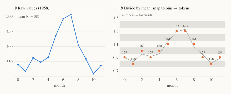
(For readability the figure uses bins of width 0.1. Real Chronos bins are about 14 times finer.)
Now a year of airline data is literally a sentence; with the figure's coarse bins, 1958 reads 159 158 160 159 160 161 163 163 161 159 158 159. The model is trained exactly like a language model, to predict the next token, with the usual cross-entropy loss. To forecast, it samples the next token, appends it, samples again, and so on for steps. Repeat that 20 times and you get 20 plausible futures. Their spread tells you how uncertain the model is.
ELI5: Chronos learned the "grammar" of time series. A rising sentence tends to keep rising; a sentence that went up-down-up every 12 words tends to keep doing that.
Patches: read a whole chunk at once#
Reading one token per time step is slow, and a single number carries very little meaning on its own, much like a single letter. Most newer models instead cut the series into patches of consecutive values. Each patch is turned into one vector (one "token") by a small neural network, and a transformer reads the sequence of patches.
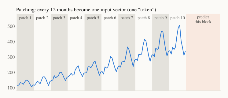
(Patch length 12 is chosen here so that one patch = one year; real models use their own fixed lengths.)
Patch-based models usually also output a whole block of future values in one go (direct multi-step forecasting, as in Part 3) instead of sampling step by step. Google's TimesFM, Salesforce's Moirai, and Amazon's own successors Chronos-Bolt and Chronos-2 all work this way. The speed gain is large: the Chronos-Bolt model card reports up to 250× faster inference than the original Chronos of the same size.
3. Forecasting a range, not a line#
All the models we test output quantiles. The -quantile is a value the future should fall below with probability . With three quantiles you can draw a fan chart:
- the median is the single best guess;
- the band between and should contain the truth about 80% of the time.
How does a network learn to output a 10th percentile? Through the pinball (quantile) loss. For one actual value and one predicted quantile :
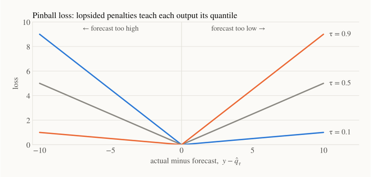
The penalty is lopsided on purpose. For , being too low costs 9 times more than being too high, so the model learns to aim high, exactly up to the point where only 10% of outcomes land above it. For the loss is symmetric and is minimised by the median. The loss with is simply half the MAE from Part 0.
A band is well calibrated if its stated coverage matches reality. An 80% band that contains the truth only 60% of the time is overconfident. We'll check this below.
4. Zero-shot on the airline data#
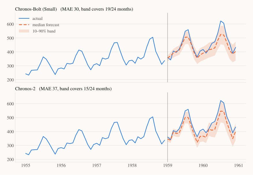
Same protocol as every other part: the context is 1949–1958 (120 months), and we forecast all 24 months of 1959–1960 in one go. Nothing is fitted. We try three open models, each of which ran in about a second on an ordinary CPU:
amazon/chronos-bolt-small(48M parameters),amazon/chronos-bolt-base(205M),amazon/chronos-2(120M).
| Method | Trained on our data? | MAE | RMSE | MAPE | MASE | 10–90% band coverage |
|---|---|---|---|---|---|---|
| Seasonal naive (Part 0) | – | 71.2 | 77.0 | 15.5% | 2.49 | – |
| Holt–Winters, multiplicative (Part 1) | yes | 29.0 | 32.5 | 6.4% | 1.01 | – |
| Linear model on lagged log-changes (Part 3) | yes | 12.1 | 15.9 | 2.8% | 0.42 | – |
| N-BEATS, small (Part 4, mean of 5 seeds) | yes | 23.5 | 28.9 | 5.1% | 0.82 | – |
| Chronos-Bolt (Small) | no | 29.6 | 38.6 | 6.0% | 1.03 | 79% |
| Chronos-Bolt (Base) | no | 38.9 | 47.5 | 8.0% | 1.36 | 71% |
| Chronos-2 | no | 37.0 | 41.6 | 7.9% | 1.29 | 62% |
What the numbers say:
- Without seeing a single training step on this series, Chronos-Bolt (Small) comes within 0.6 (thousand passengers) of Holt–Winters on MAE and beats it on MAPE. All three models cut the seasonal naive error roughly in half or better. That is the promise of the era, and it holds.
- None of them clearly beats a well-specified Holt–Winters here, and models fitted to this series (Part 3's linear model, Part 4's N-BEATS) do better still. This series is short, clean, and exactly the shape that classic methods were designed for.
- All three underestimate the 1960 summer peak. The Chronos authors flagged exactly this case: in their paper they show Air Passengers with 120 observations of context and a 24-month horizon, and note that the original Chronos "tends to underestimate trend" when the context is short (Figure 13 of Ansari et al., 2024).
- Bigger is not automatically better. Bolt-Base has four times the parameters of Bolt-Small and does worse on this series. One series is one draw; never pick a model from a single result.
- The bands are a bit too narrow. An 80% band should cover about 19 of 24 months. Bolt-Small manages 19, Bolt-Base 17, and Chronos-2 only 15, mostly missing the high summer months.
5. The landscape, briefly#
The field moves fast, so here are only the well-established families, each linked to its paper:
| Model | From | Key idea | Open weights? |
|---|---|---|---|
| TimeGPT | Nixtla, 2023 | transformer offered as a commercial forecasting service | no, API only |
| Lag-Llama | open research collaboration, 2023 | small decoder-only model fed with lagged values; outputs a probability distribution | yes |
| TimesFM | Google, 2023 | decoder-only, patches in, longer patches out; latest open release is TimesFM 2.5 (200M) | yes |
| Moirai | Salesforce, 2024 | "any-variate" masked encoder that handles many series and frequencies at once; Moirai 2.0 is non-commercial (CC BY-NC 4.0) | yes |
| Chronos / Chronos-Bolt | Amazon, 2024 | tokens and a T5 language model; Bolt switches to patches and direct quantiles (9M–205M) | yes |
| Chronos-2 | Amazon, 2025 | adds multivariate inputs and covariates; context up to 8,192 steps | yes |
Two public leaderboards, GIFT-Eval and fev-bench, compare these models across many datasets. They are the right place to check current rankings, which change every few months.
Zero-shot or fine-tune? Start zero-shot: it costs nothing and gives you a strong baseline in minutes. Fine-tune when you have plenty of series from a domain that looks unlike the pretraining data (sensor readings with unusual dynamics, for example) and you have measured that zero-shot falls short.
6. In code#
Zero-shot forecasting really is a few lines:
import numpy as np, torch
import statsmodels.api as sm
from chronos import BaseChronosPipeline

y = sm.datasets.get_rdataset("AirPassengers").data["value"].to_numpy(dtype=float)
train, test = y[:120], y[120:]                       # 1949–1958 | 1959–1960

pipe = BaseChronosPipeline.from_pretrained("amazon/chronos-bolt-small", device_map="cpu")
q, _ = pipe.predict_quantiles(torch.tensor(train), prediction_length=24,
                              quantile_levels=[0.1, 0.5, 0.9])
lo, med, hi = q[0].numpy().T                         # each holds 24 monthly values

print(f"MAE={np.abs(test - med).mean():.1f}  "
      f"80% band covers {np.mean((test >= lo) & (test <= hi)):.0%} of months")
MAE=29.6 80% band covers 79% of months
(pip install chronos-forecasting; the model weights download from the Hugging Face Hub on first use.)
7. Where foundation models run out#
- Test leakage is a real risk. A zero-shot score means little if the model saw the test data during pretraining. For our data the news is reasonably good but not airtight. Air Passengers is not among the training datasets listed in the Chronos paper, though the same paper uses it as an example. The TimesFM paper reports results on Air Passengers as part of the Darts benchmark. Chronos-2 adds a large synthetic corpus plus public collections. And a dataset this famous has been copied into countless repositories. Benchmarks now track this explicitly: in the Chronos-2 report's fev-bench table, the share of tasks flagged as overlapping with a model's training data ranges from 0% to 28% depending on the model. Always validate on your own, recent, private data.
- Compute. About a second per series on a CPU is fine for one series, but Holt–Winters takes milliseconds. For millions of series, or forecasts on a small device, that gap matters.
- Context length. Each model has a maximum context (512 steps for the original Chronos, 2,048 for Chronos-Bolt, 8,192 for Chronos-2). And as we saw, short context hurts too: 120 months was not enough to pin down the trend.
- Covariates. Most models see only the history of the series itself. Promotions, holidays and prices need either a model built for covariates (Chronos-2 is one) or a separate regression on top.
- Opacity and licences. You can't inspect a level, a slope and a seasonal factor as you can with Holt–Winters, and some weights (Moirai 2.0, for example) can't be used commercially.
So when should you still prefer Holt–Winters? When the series is short, regular and clearly seasonal, when you need to explain every number to a stakeholder, or when compute is tight. When should you reach for a foundation model? When you have many diverse series and little time to tune a model for each, when you need a strong baseline today, or when you want calibrated ranges without building a probabilistic model yourself.
Recap#
- A foundation model is pretrained once on billions of observations and then forecasts new series zero-shot: your history is the prompt, nothing is fitted.
- Chronos turns numbers into words: mean scaling , then binning into 4,094 tokens, then a language model. Patch-based models (TimesFM, Moirai, Chronos-Bolt, Chronos-2) read chunks of values and output whole blocks of future values, which is much faster.
- They output quantiles, learned with the lopsided pinball loss; check that the 80% band really covers about 80%.
- Zero-shot on the airline data, Chronos-Bolt (Small) matches Holt–Winters (MAE 29.6 vs 29.0) with no training. No model clearly wins, and the bands are slightly too narrow.
- Watch for test leakage, context limits, missing covariates and licences.
Next up — Part 6: The showdown. We have now met five eras of forecasting. In the final part we put every method from the series side by side on the same data and finish with a practical guide: given your problem, which one should you reach for first?