
Time Series, Era by Era — Part 4: Deep Learning, Letting the Network Find the Features
November 5, 2026 · 9 min read · Time Series, Forecasting, Deep Learning
Contents · 6 sections
- 1. From a series to training examples
- Windows
- Normalisation: make every window look alike
- 2. A quick tour of the architectures
- MLP: the plain neural forecaster
- RNN / LSTM: reading the series like a sentence
- TCN: convolutions that look far back
- N-BEATS: blocks that explain and pass on
- DeepAR, in one sentence
- Transformers, and the linear model that embarrassed them
- 3. The experiment
- 4. In code
- 5. Where deep learning runs out
- Recap
In Part 3 we forecast by hand-crafting features: lags, rolling means, calendar flags. That works, but you decide what the model gets to see. If you forget the 12-month lag, the model never learns about summers.
Deep learning flips this around. Think of the difference between giving someone a checklist ("look at last month, last year, the 3-month average") and handing them the raw chart and saying "you figure out what matters." A neural network gets the raw recent history and learns its own features from the data.
This post covers:
- how to turn one series into training examples a network can learn from,
- a quick, intuition-only tour of the main architectures (MLP, LSTM, TCN, N-BEATS, Transformers),
- an honest experiment on our airline data, including a surprising result about linear models.
1. From a series to training examples#
Windows#
A network needs many (input, target) pairs. We cut them from the series with a sliding window: the last months are the input, the next months are the target, then we slide one month and repeat.
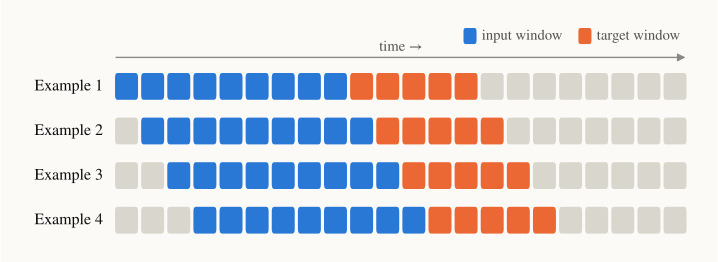
We use (three years of history) and (the two test years, predicted in one shot). Predicting all steps at once is called direct multi-output forecasting. Unlike predicting one step and feeding it back in, mistakes don't snowball. From our 120 training months this gives only 61 windows. Keep that number in mind.
Normalisation: make every window look alike#
A window from 1950 (around 150 passengers) and one from 1958 (around 400) have the same shape but very different scale. A network would waste its capacity learning that they're related. Two cheap tricks fix this:
- Take logs, . Multiplicative seasonality ("+20% in July", see Part 0) becomes additive ("+0.18 in July").
- Re-centre each window on its last value. For a window that ends at time , the input and target are
Now every input ends at 0, and the target reads as "how much higher or lower than today, in log units (roughly percent)." To forecast, feed in the last 36 months and undo both steps:
Here is the network with weights , and is its -th output. Training minimises the mean squared error between and over all windows. Honestly, this unglamorous preprocessing does as much work as any architecture below.
2. A quick tour of the architectures#
MLP: the plain neural forecaster#
A multi-layer perceptron treats the 36 inputs as a flat list and passes them through a few dense layers:
are weight matrices, bias vectors, and (ReLU) is the bend that lets the model learn non-linear patterns. Ours has two hidden layers of 64 units. It doesn't know that input 35 comes right after input 34; it just learns which positions matter.
RNN / LSTM: reading the series like a sentence#
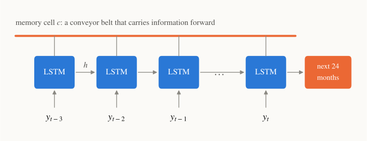
A recurrent network reads the window one month at a time and keeps a running summary, the hidden state , like you keep the plot in mind while reading a book. Plain RNNs forget quickly. The LSTM (Hochreiter & Schmidhuber, 1997) adds a memory cell , a conveyor belt that information can ride along almost untouched:
The forget gate decides how much old memory to keep, the input gate how much of the new candidate to write, and is element-wise multiplication. All gates are small learned layers that look at the current input and previous hidden state.
TCN: convolutions that look far back#
A temporal convolutional network (Bai et al., 2018) slides small filters along time instead. Two tweaks make it suit forecasting. The filters are causal (each output only sees the past), and they are dilated: layer skips steps, with
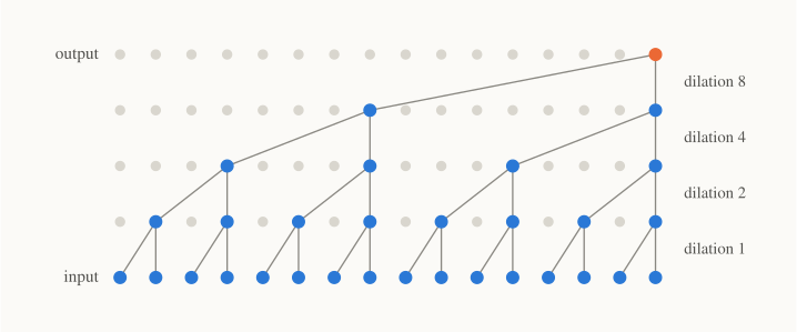
With filter size , the output sees past steps. The reach doubles with every layer, so a few layers cover a long history cheaply. Like a family tree, each generation back covers twice as many ancestors.
N-BEATS: blocks that explain and pass on#
N-BEATS (Oreshkin et al., 2020) beat the winner of the M4 forecasting competition using nothing but stacks of MLP blocks. Each block outputs two things: a backcast (its explanation of the input) and a forecast . The next block only sees what is still unexplained:
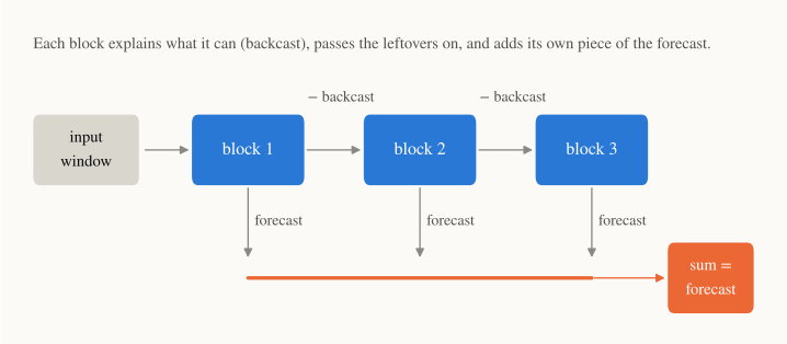
ELI5: a team of painters, where each one paints what they can see is missing and hands the canvas on. In the "interpretable" version, one stack may only paint smooth polynomials (trend) and another only sine waves (seasonality). That's the decomposition from Part 0, learned end-to-end.
DeepAR, in one sentence#
DeepAR (Salinas et al., 2020, Amazon) is an LSTM that outputs a probability distribution for each future step instead of a single number, trained across thousands of related products at once. That "one model, many series" idea will matter a lot in Part 5.
Transformers, and the linear model that embarrassed them#
Transformers use attention: every position looks at every other position and decides which ones are relevant, like scanning the whole chart for the months that resemble now. After their success in language, a wave of time-series Transformers followed (Informer, Autoformer, FEDformer, …).
Then Zeng et al. (2023) asked the awkward question "Are Transformers effective for time series forecasting?" They proposed DLinear: split the window into a moving-average trend and a remainder, and map each to the forecast with one linear layer:
This model has no hidden layers and no attention, and it beat all those Transformers on the standard long-horizon benchmarks.
Part of the problem was tokens. Feeding one time point per token is like reading a book one letter at a time: a single number says almost nothing on its own. PatchTST (Nie et al., 2023) fixed this by grouping consecutive points into patches, short sub-series that become the tokens:
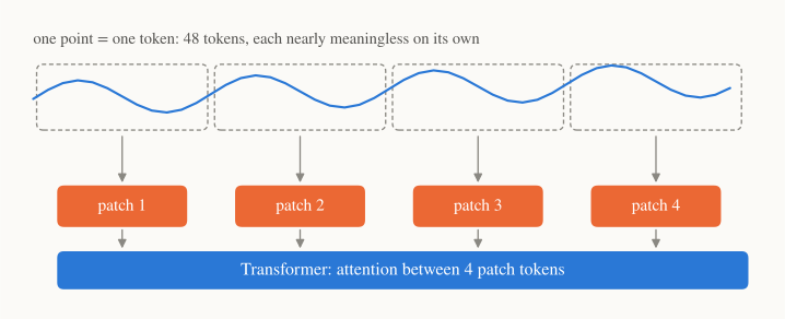
With patch length and stride , a window of points becomes tokens. Each token now carries a local shape (a rise, a dip), and attention, whose cost grows like , gets much cheaper. Patching put Transformers back on top of the benchmarks, and it is the backbone of most foundation models in Part 5.
We won't train a Transformer here: with 61 training windows it would mostly memorise noise.
3. The experiment#
Same split as every part: train on 1949–1958, forecast all of 1959–1960. Four small models, all on the log-and-re-centre windows from Section 1:
| Model | Parameters | Notes |
|---|---|---|
| DLinear | 1,776 | moving-average kernel 13, two linear maps |
| MLP | 8,088 | 2 hidden layers × 64 units |
| LSTM | 5,272 | 32 hidden units, last hidden state → 24 outputs |
| N-BEATS (small) | 31,284 | 3 generic blocks, 2 layers × 64 units each |
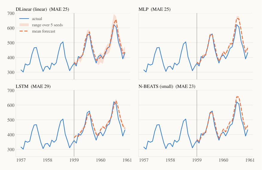
All are trained with Adam (learning rate , weight decay ) for 600 full-batch epochs. That takes under a second per model on a laptop CPU. The settings were picked once and not tuned on the test years. Neural networks start from random weights, so each model is trained with 5 different seeds and we report the average and the range.
| Method | MAE | RMSE | MAPE | MASE | MAE range (5 seeds) |
|---|---|---|---|---|---|
| Seasonal naive (Part 0) | 71.2 | 77.0 | 15.5% | 2.49 | – |
| Holt–Winters (Part 1) | 29.0 | 32.5 | 6.4% | 1.01 | – |
| Linear model on lagged log-changes (Part 3) | 12.1 | 15.9 | 2.8% | 0.42 | – |
| DLinear (linear) | 25.0 | 30.9 | 5.4% | 0.88 | 23.0–28.4 |
| MLP | 25.2 | 31.0 | 5.5% | 0.88 | 22.3–28.7 |
| LSTM | 29.1 | 35.0 | 6.8% | 1.02 | 26.1–36.1 |
| N-BEATS (small) | 23.5 | 28.9 | 5.1% | 0.82 | 21.5–26.2 |
How to read this honestly:
- The networks are in the same league as Holt–Winters, not far ahead of it. The seed ranges (about ±3 MAE) are as wide as the gaps between models, and we have only one 24-month test window. "N-BEATS wins" would be over-reading the table.
- The linear model keeps up with the MLP. That's the DLinear lesson in miniature: once the windows are well normalised, a linear map captures most of what this series has to offer.
- And Part 3's plain linear regression still beats every network (MAE 12.1). It works on month-to-month log-changes, a representation that already strips out the growth. The networks have to learn that from 61 windows. On one small series, choosing the right representation matters more than choosing the architecture.
- The LSTM is the weakest and the most seed-sensitive (26 to 36). Reading 36 steps one at a time to predict 24 at once is a harder learning problem than looking at all 36 together.
- All models overshoot the 1960 peak. They learned "summers keep getting bigger" a little too eagerly from a handful of examples.
- Note the parameter counts: every network has more weights than there are numbers in our training targets (61 × 24 = 1,464). Weight decay and the short training keep this from becoming pure memorisation. But on a single small series, we're near the edge of what these models should be trusted with.
4. In code#
The whole MLP pipeline, from windows and training to forecast, in PyTorch:
import numpy as np, torch, statsmodels.api as sm
from torch import nn

y = np.log(sm.datasets.get_rdataset("AirPassengers").data["value"].to_numpy(float))
train, test = y[:120], np.exp(y[120:])           # log scale | original scale
L, H = 36, 24                                    # look back 3 years, predict 2

# sliding windows over the training years, each re-centred on its last input
starts = range(len(train) - L - H + 1)
X = torch.tensor(np.array([train[s:s+L] - train[s+L-1] for s in starts]), dtype=torch.float32)
Y = torch.tensor(np.array([train[s+L:s+L+H] - train[s+L-1] for s in starts]), dtype=torch.float32)

torch.manual_seed(0)
model = nn.Sequential(nn.Linear(L, 64), nn.ReLU(), nn.Linear(64, 64), nn.ReLU(), nn.Linear(64, H))
opt = torch.optim.Adam(model.parameters(), lr=1e-3, weight_decay=1e-4)
for epoch in range(600):
    opt.zero_grad()
    loss = nn.functional.mse_loss(model(X), Y)
    loss.backward()
    opt.step()

x = torch.tensor(train[-L:] - train[-1], dtype=torch.float32)
forecast = np.exp(model(x).detach().numpy() + train[-1])
print(f"MAE = {np.abs(test - forecast).mean():.1f}")
This prints MAE = 24.1 for seed 0, one of the five runs behind the MLP row above.
5. Where deep learning runs out#
- Data hunger. One series of 144 months is the worst case for neural nets. They shine when you train one global model on many related series (thousands of products, sensors, stores), so patterns learned on one help the others. That's what DeepAR and N-BEATS were built for.
- More knobs, more variance. Window length, normalisation, architecture, learning rate, epochs and seeds all move the result. Holt–Winters has three parameters and gives the same answer every time.
- Cost and care. Seconds instead of milliseconds here, and GPUs and real engineering at scale.
- Still one dataset at a time. Each model above starts from zero knowledge of what time series look like. It has to rediscover "seasons repeat" and "trends continue" from 61 examples.
That last point raises the obvious question: what if a model had already seen millions of series before it ever met ours?
Recap#
- Neural forecasters learn their own features from raw windows of recent history; direct multi-output predicts all steps at once.
- Logs plus per-window re-centring make windows from different eras comparable, and matter as much as the architecture.
- MLP sees the window as a flat list, LSTM reads it step by step with a memory cell, TCN uses dilated causal convolutions, and N-BEATS stacks blocks that explain and pass on residuals.
- Transformers needed patching (PatchTST) to work well. Meanwhile DLinear, one linear layer, showed that many complex models weren't earning their complexity.
- On our 120-month series, tiny networks match Holt–Winters within seed noise. Deep learning pays off with many series, not one.
Next up — Part 5: Foundation models. What if we pretrain one big model on a huge collection of real time series, then ask it to forecast airline passengers it has never seen, with no training at all? That's the idea behind Chronos, TimesFM and Moirai, and the newest era of forecasting.