
Time Series, Era by Era — Part 3: Machine Learning, or Turning a Series into a Table
November 5, 2026 · 8 min read · Time Series, Forecasting, Machine Learning
Contents · 11 sections
- 1. From a series to a table
- 2. The feature menu
- 3. The leakage trap in rolling features
- 4. Trees can't extrapolate a trend
- The fix: predict the change, not the level
- 5. Forecasting many steps: recursive vs direct
- 6. Two models on the same table
- 7. Results
- What did the trees learn?
- 8. Where trees really shine: many series at once
- 9. In code
- 10. Where it runs out
- Recap
Imagine a friend who is brilliant with spreadsheets but has never heard of time. Give them a table where each row has some inputs and one answer, and they'll find the pattern: linear regression, random forests, gradient boosting, you name it. Give them a time series, and they don't know what to do with it.
The whole trick of this era is a translation: turn the series into a table, hand it to a standard machine-learning model, and turn the model's answers back into a forecast. It sounds almost too simple, but gradient-boosted trees built this way dominated the big M5 forecasting competition in 2020, and they run a large share of real-world demand forecasting today.
We keep the setup from earlier parts: monthly airline passengers, train on 1949–1958, forecast all 24 months of 1959–1960, and compare with the Part 0 baselines and Holt–Winters.
1. From a series to a table#
Pick a window of the last values. Those are the features; the value right after the window is the target. Then slide the window forward one step and repeat:
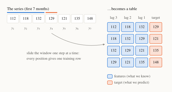
In symbols, the row for time is
where is called lag : the value steps before . A machine-learning model learns a function such that
Look at the figure again: 7 months give training rows with . In general a series of length gives rows. For our airline training set that means about 107 rows. This number matters later: it's tiny by machine-learning standards.
2. The feature menu#
Lags are only the start. Because it's "just a table," you can add any column that you'd know at the time of forecasting:
| Feature | Example | What it captures |
|---|---|---|
| Recent lags | momentum, short-term level | |
| Seasonal lag | (monthly), (daily) | "same time last cycle" |
| Rolling statistics | mean / std of the last 12 values | local level and volatility |
| Calendar | month, day of week, holiday flag | fixed seasonal and calendar effects |
| External (exogenous) | price, promotion, weather forecast | causes from outside the series |
That last row is a big deal. Smoothing methods (Part 1) can't use a promotion calendar at all. Here it's simply one more column.
For the airline data we use 14 features: lags 1 to 12, the mean of the last 12 values, and the calendar month.
3. The leakage trap in rolling features#
Rolling features hide the most common bug in this whole field. Compare two ways of computing a "rolling mean of 4 months" for the row that predicts month :
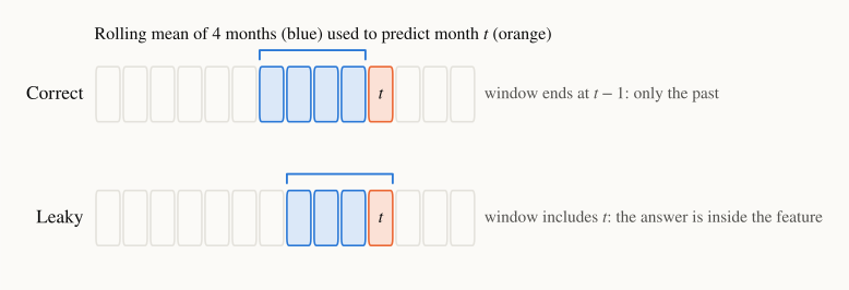
The correct version uses only values strictly before :
The leaky version starts the sum at , so it includes , the very value we want to predict. During training the model happily learns "the target is roughly the rolling mean," and validation scores look superb. At forecast time doesn't exist yet, so the feature can't even be computed honestly. In pandas, the fix is one word: y.shift(1).rolling(w).mean(), not y.rolling(w).mean().
Rule of thumb: for every column, ask "would I really know this value at the moment I make the forecast?"
4. Trees can't extrapolate a trend#
Now train LightGBM on the raw passenger counts and forecast 1959–1960. The forecast gets the seasonal shape but never climbs above about 500 passengers, even though the real peaks go past 600:
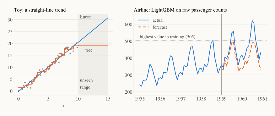
The left panel shows why, on a toy straight line. A decision tree splits the input space into regions and predicts the average training target in each region. So its prediction can never leave the range of targets it has seen:
A boosted ensemble of trees is a sum of such pieces and stays stuck in practice too. In our airline training data the highest value is 505, and the forecast plateaus just below it. Linear models don't have this problem: a line keeps going.
The fix: predict the change, not the level#
ELI5: don't ask "how tall will the child be next year?" Ask "how much will the child grow?" Growth looks similar every year, even though the height keeps increasing.
We model the monthly log-change
which is approximately the percentage change from the previous month (for small changes, ). Unlike passenger counts, these changes don't trend upward, so every future value lies in a range the model has already seen. After predicting changes , we rebuild the level:
The log also handles the "swings grow with the level" pattern from Part 0: a fixed percentage swing becomes a fixed-size swing in .
5. Forecasting many steps: recursive vs direct#
A one-step model predicts . How do we get all 24 months?
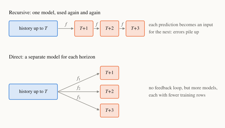
Recursive: train one model for one step ahead. Predict , append the prediction to the history as if it were real, predict , and so on:
It's simple and needs only one model, but any mistake is fed back as input, so errors can snowball. It's like a game of telephone with yourself.
Direct: train a separate model for each horizon , always using only real history:
There's no feedback loop, but now we need 24 models. Each also has fewer usable rows, because a row needs its answer steps in the future: 107 rows for shrink to 84 for .
6. Two models on the same table#
- Linear regression: . Fit by least squares.
- LightGBM, a gradient-boosted tree ensemble. It builds trees one after another, each small tree fitting the errors left by the previous ones, and adds them up with a learning rate :
We use trees with at most 8 leaves each, , and at least 5 rows per leaf (the default of 20 is too many for 107 rows). The settings were fixed up front, not tuned on the test years.
7. Results#
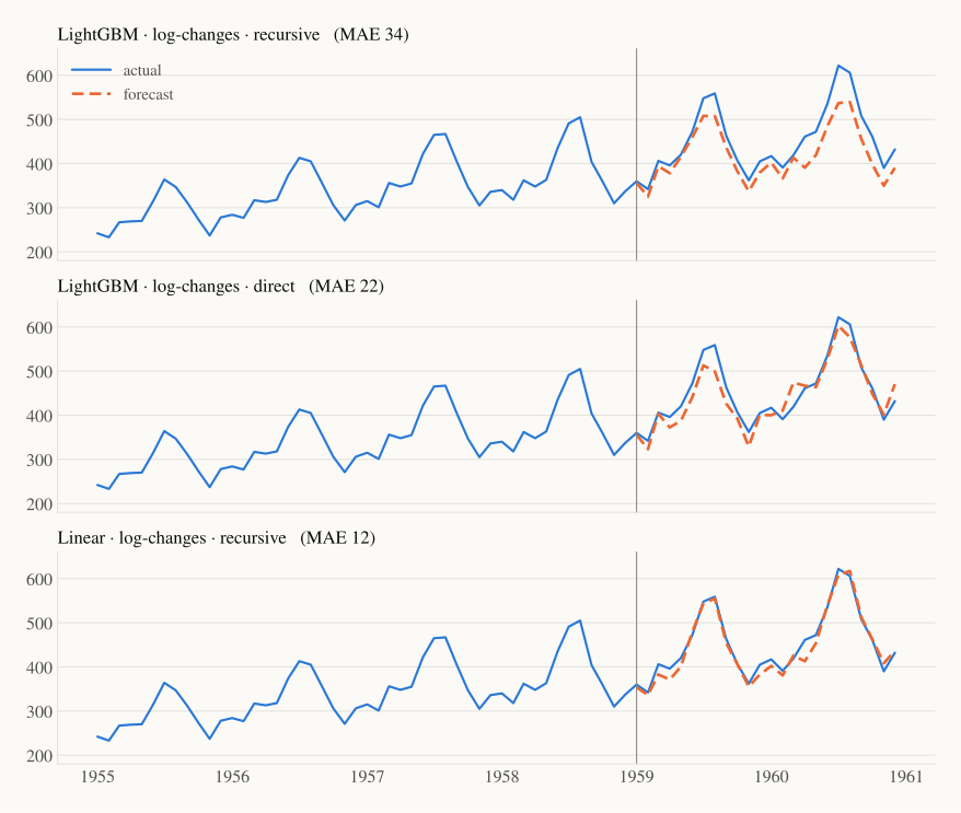
| Method | MAE | RMSE | MAPE | MASE |
|---|---|---|---|---|
| Seasonal naive (Part 0) | 71.2 | 77.0 | 15.5% | 2.49 |
| Holt–Winters, multiplicative (Part 1) | 29.0 | 32.5 | 6.4% | 1.01 |
| LightGBM · raw levels · recursive | 54.8 | 64.0 | 11.7% | 1.92 |
| LightGBM · log-changes · recursive | 34.4 | 41.1 | 7.2% | 1.21 |
| LightGBM · log-changes · direct | 21.9 | 26.9 | 4.9% | 0.77 |
| Linear · log-changes · recursive | 12.1 | 15.9 | 2.8% | 0.42 |
Reading top to bottom:
- Raw LightGBM is capped by its own training range: better than seasonal naive, far worse than Holt–Winters.
- Predicting log-changes removes the cap: MAE falls from 54.8 to 34.4.
- Going direct stops the error snowball and beats Holt–Winters (21.9 vs 29.0).
- The plain linear model wins. With 14 features and only 107 rows, flexibility is a liability: trees spend their capacity carving the data into small boxes, while a straight line on well-chosen features is exactly the right amount of model. A linear regression on lagged log-changes is essentially an autoregressive model, close to the seasonal ARIMA from Part 2b. The new era didn't make the old ideas wrong. They became a special case.
Keep the scale in mind: this is one small series and a single 24-month test window. Small changes in settings can reorder the middle rows. The robust lessons are the mechanisms (extrapolation, transformation, error feedback), not the exact ranks.
What did the trees learn?#
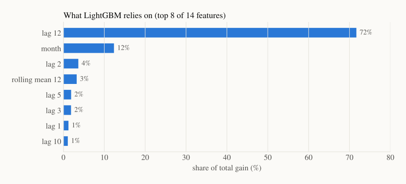
Gain importance measures how much each feature reduced the training error, summed over all the splits that used it. Lag 12 alone accounts for 72%, and the month for another 12%. Nobody told the model about seasons. It rediscovered "this month looks like the same month last year," which is exactly the seasonal naive idea from Part 0, now learned from data.
8. Where trees really shine: many series at once#
On a single series of 120 points, gradient boosting is fighting with one hand tied. Its home ground is global models: one model trained on thousands of related series at once (every product in every store), with extra columns such as product category, store or price.
- The table gets millions of rows instead of 107.
- Patterns are shared: a new product can borrow seasonality learned from similar ones.
- Exogenous features (promotions, holidays, prices) carry real signal.
That's the story of the M competitions. In M4 (2018), pure machine-learning entries mostly lost to statistical methods. In M5 (2020), which asked for forecasts of about 30,000 Walmart product–store series with prices and calendar events, LightGBM-based global models took the top places. The method didn't change between the two; the data setting did.
9. In code#
The linear and LightGBM rows from the table, recursive strategy on log-changes:
import numpy as np, lightgbm as lgb
import statsmodels.api as sm
from sklearn.linear_model import LinearRegression

y = sm.datasets.get_rdataset("AirPassengers").data["value"].to_numpy()
train, test = y[:120], y[120:]                      # 1949–1958 | 1959–1960
d = np.diff(np.log(train))                          # monthly log-changes
month = np.arange(1, 120) % 12 + 1                  # calendar month of each change

def row(hist, m):                                   # lag 1..12, rolling mean, month
    h = np.asarray(hist)[-12:]
    return [*h[::-1], h.mean(), m]

X = np.array([row(d[:t], month[t]) for t in range(12, len(d))])
Y = d[12:]

for name, model in [("linear", LinearRegression()),
                    ("lightgbm", lgb.LGBMRegressor(n_estimators=300, learning_rate=0.05, num_leaves=8,
                                                   min_child_samples=5, random_state=0, verbose=-1))]:
    model.fit(X, Y)
    hist, log_level, preds = list(d), np.log(train[-1]), []
    for h in range(24):                             # recursive: feed each prediction back in
        step = model.predict(np.array([row(hist, h % 12 + 1)]))[0]
        hist.append(step)
        log_level += step
        preds.append(np.exp(log_level))
    print(f"{name:9s} MAE={np.mean(np.abs(test - np.array(preds))):.1f}")
Output: linear MAE=12.1 and lightgbm MAE=34.4.
10. Where it runs out#
- You are the feature engineer. Which lags? Which windows? Which holidays? Every choice is manual, and a missing feature is invisible to the model.
- Trees don't extrapolate. You must remember to detrend or difference, then undo it.
- Multi-step is awkward. Recursive forecasts snowball errors; direct forecasts multiply models.
- Order is only as deep as your lags. The model sees a flat row of numbers, not a sequence. A pattern 18 months back doesn't exist unless you added lag 18.
The obvious next question: could a model learn the features itself, straight from the raw sequence?
Recap#
- Turn a series into a table: lags, rolling stats, calendar and external features become columns; the next value is the target.
- Shift before you roll. Every feature must be known at forecast time.
- Trees can't extrapolate. Predict changes (e.g. log-differences) and rebuild the level.
- Recursive = one model, errors feed back. Direct = one model per horizon, fewer rows each.
- On one small series, a linear model on good features (12.1 MAE) beat LightGBM and Holt–Winters. Trees shine as global models across thousands of series, as in M5.
Next up — Part 4: Deep learning. Instead of hand-crafting lags and windows, we let neural networks read the sequence directly: recurrent networks that carry a memory forward, convolutions that scan for patterns, and N-BEATS and Transformers that learn trend and seasonality on their own.