
Time Series, Era by Era — Part 2a: Does Today Echo Yesterday?
November 5, 2026 · 8 min read · Time Series, Forecasting, Statistics
Contents · 9 sections
- 1. Stationarity: the rules don't change over time
- 2. Making a series stationary: log and differencing
- Can we test for it?
- 3. Autocorrelation: measuring the echo
- The ACF plot
- The PACF: the direct echo
- 4. AR models: today is a weighted sum of the past
- 5. MA models: today remembers yesterday's surprises
- 6. Telling AR and MA apart: ACF and PACF signatures
- 7. In code
- Where these tools run out
- Recap
Shout into a canyon and the sound comes back: loud at first, then fainter, then gone. Many time series behave the same way. A hot day tends to be followed by another warm day, and a big sales week leaves a little bump in the next one. The past echoes into the present.
Part 1 described a series by its components: a level, a slope and a seasonal pattern. In the 1970s, George Box and Gwilym Jenkins popularised a different view: describe a series by how strongly, and for how long, each value echoes into the next ones. Their model family is ARIMA, still one of the most widely used forecasting tools today.
ARIMA has enough moving parts that we'll take it in two posts:
- Part 2a (this post): the building blocks: stationarity, differencing, autocorrelation, and the AR and MA models.
- Part 2b: putting them together into (S)ARIMA, fitting it to the airline data, and producing forecasts with uncertainty bands.
1. Stationarity: the rules don't change over time#
To learn "how today echoes yesterday," that echo has to be the same in 1950 and in 1960. Otherwise there's no single pattern to learn. That's the idea behind stationarity.
A series is (weakly) stationary if:
- its mean doesn't change over time;
- its variance (spread) doesn't change over time;
- the correlation between and depends only on the gap , not on when you look.
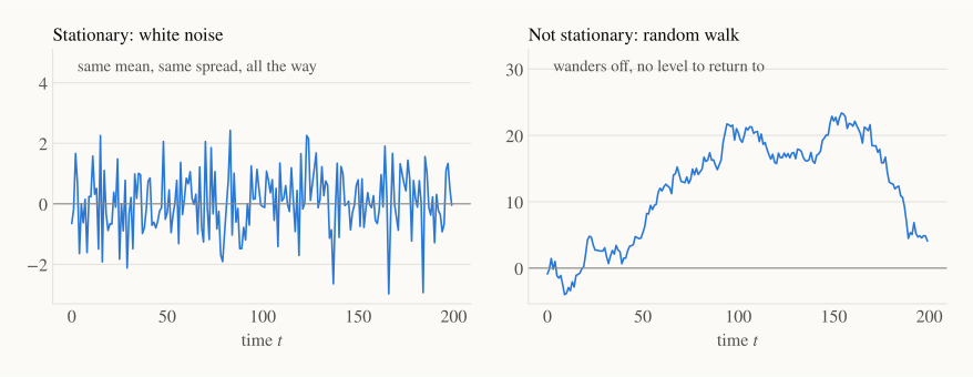
Two series that come up again and again:
White noise is the simplest stationary series: independent random shocks with mean 0 and a fixed variance .
It has no echo at all: knowing today tells you nothing about tomorrow. It's the "nothing left to learn" baseline.
Random walk: today equals yesterday plus a fresh shock.
Every shock is kept forever, so the series wanders off and never returns to any level. Stock prices behave roughly like this. A random walk is not stationary, because its variance keeps growing with time.
The airline series from Part 0 breaks all the rules: its mean rises (trend), its spread grows, and its pattern repeats every 12 months. So before ARIMA can use it, we need to make it stationary.
2. Making a series stationary: log and differencing#
There are two simple tools.
Log fixes growing swings. Taking turns a multiplicative pattern ("+20% every July") into an additive one ("+0.18 every July").
Differencing removes a trend. Instead of the values, look at the changes:
The first five airline months are 112, 118, 132, 129, 121. Their differences are
The trend is gone: a steadily rising series turns into changes that hover around a constant. (Notice that a random walk becomes white noise after one difference: .)
Seasonal differencing removes a repeating yearly pattern by comparing each month with the same month last year:
For example, January 1950 minus January 1949 is .
Applying these steps one after another to the airline data:
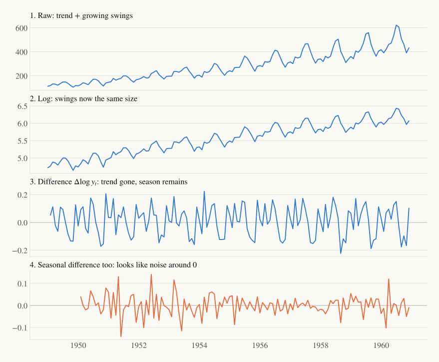
After log + difference + seasonal difference, what's left looks like noise around zero, which is what we want. The number of ordinary differences is called and the number of seasonal differences . Here and , and they become the "I" (for integrated) in ARIMA.
Can we test for it?#
Yes. Two classic tests give a second opinion beyond eyeballing:
- ADF (augmented Dickey–Fuller): null hypothesis "not stationary." A small p-value says stationary.
- KPSS: the opposite null, "stationary." A small p-value says not stationary.
On the training data (1949–1958), the raw series gets ADF and KPSS : both say not stationary. After log + difference + seasonal difference, ADF and KPSS : both say stationary. When the two tests agree, you can be fairly confident.
3. Autocorrelation: measuring the echo#
How strongly does a series echo itself steps later? The autocorrelation at lag is the ordinary correlation between the series and a copy of itself shifted by steps:
Here is the mean of the series. The numerator asks "when was above average, was above average too?" The denominator scales the result to lie between and .
A tiny worked example. Take , so and the deviations are .
- Denominator: .
- Numerator for , multiplying each deviation by the one before it: .
- So : a moderate positive echo. Above-average values tend to follow above-average values.
The ACF plot#
Plot for and you get the autocorrelation function (ACF), also called a correlogram. Each stick is one lag. The grey band, , marks how big a correlation could be by pure chance if the series were white noise. Sticks inside the band are "no real echo"; sticks poking out are signal.
For the raw airline series, the ACF starts at and decays very slowly (). That slow decay is the fingerprint of a trend, another sign that the series needs differencing.
The PACF: the direct echo#
There's a catch. If today echoes yesterday, and yesterday echoed the day before, then today will also correlate with the day before, just indirectly, passed along through yesterday. The ACF can't tell direct and indirect echoes apart.
The partial autocorrelation function (PACF) at lag measures the correlation between and after removing the effect of the lags in between (). ELI5: the ACF hears every echo in the canyon; the PACF only hears the sound that bounces straight back from the wall steps away.
4. AR models: today is a weighted sum of the past#
An autoregressive model of order , written AR(), says that today is a weighted sum of the last values plus a fresh shock:
- is a constant,
- are the AR coefficients (how much each past value carries over),
- is white noise: the part nobody could have predicted.
It's literally a linear regression of the series on its own past, hence auto-regressive. The simplest case, AR(1), shows what the coefficient does:
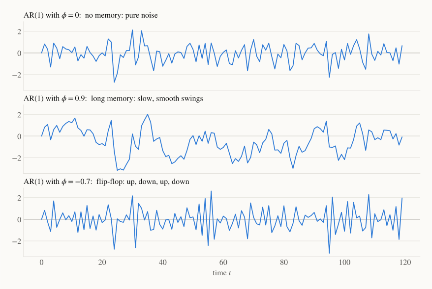
- : no memory, so the series is white noise.
- : strong memory. Shocks fade slowly, producing long, smooth swings.
- : today tends to have the opposite sign of yesterday, so the series zig-zags.
For AR(1) to be stationary we need , so shocks die out. At we're back to the random walk, where shocks live forever. AR(1)'s ACF is : the echo fades geometrically, just like the weights of exponential smoothing in Part 1.
5. MA models: today remembers yesterday's surprises#
A moving-average model of order , written MA(), says that today depends on the last shocks, not the last values:
- is the mean,
- are the MA coefficients,
- are past surprises (past forecast errors).
ELI5: a local TV segment mentions your coffee shop. That surprise lifts sales today and a little tomorrow, then everyone forgets. An MA() process has a short, finite memory: a shock matters for exactly steps and then disappears completely. (Despite the name, this has nothing to do with the moving-average smoother of Part 1.)
6. Telling AR and MA apart: ACF and PACF signatures#
Here's the practical payoff. AR and MA processes leave opposite fingerprints in the ACF and PACF:
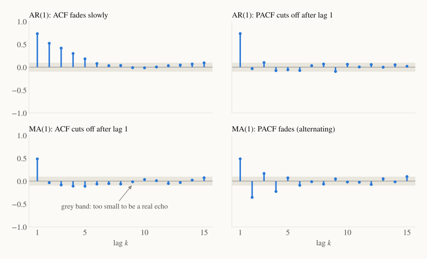
| ACF | PACF | |
|---|---|---|
| AR() | fades gradually | cuts off after lag |
| MA() | cuts off after lag | fades gradually |
Why? In AR(1), each value passes its echo along to the next, so correlations fade slowly (ACF), but the only direct link is to lag 1 (PACF). In MA(1), a shock only lives one step, so values more than one step apart share nothing (ACF cuts off). The PACF has to untangle that, and it fades instead.
Real data is noisier than these clean simulations, and you'll often see patterns that are a bit of both. That's when we'll let the computer compare candidate models, which is exactly where Part 2b picks up.
7. In code#
Everything in this post is a one-liner in statsmodels:
import numpy as np
import statsmodels.api as sm
from statsmodels.tsa.stattools import acf, adfuller

y = sm.datasets.get_rdataset("AirPassengers").data["value"].to_numpy()[:120]  # 1949–1958
d = np.diff(np.log(y))                       # log, then difference
z = d[12:] - d[:-12]                         # then seasonal difference (lag 12)

print(f"raw: ADF p={adfuller(y)[1]:.3f}  r1={acf(y, nlags=1)[1]:.2f}")
print(f"z:   ADF p={adfuller(z)[1]:.3f}  r1={acf(z, nlags=12)[1]:.2f}  r12={acf(z, nlags=12)[12]:.2f}")
raw: ADF p=0.827  r1=0.94
z:   ADF p=0.001  r1=-0.33  r12=-0.41
Those last two numbers, the clear echoes at lag 1 and lag 12 in the stationary series, are exactly the clues we'll use to choose a model in Part 2b.
Where these tools run out#
- Linear echoes only. AR and MA capture linear relationships with the past. They can't say "a heatwave matters only when it's also a weekend."
- Stationarity is required. Differencing works for simple trends and seasons, but sudden breaks (a pandemic, a policy change) violate the "rules don't change" assumption.
- Reading ACF/PACF is part art. The clean signatures above get muddy on short, noisy real data.
Recap#
- Stationary = constant mean, constant variance, and an echo that depends only on the lag. White noise is stationary; a random walk is not.
- Use log to stabilise growing swings, differencing () to remove trends and seasonal differencing () to remove yearly patterns. Check with ADF and KPSS.
- ACF measures the total echo at each lag; PACF measures the direct echo.
- AR() regresses on past values: ACF fades, PACF cuts off at .
- MA() remembers past shocks: ACF cuts off at , PACF fades.
Next up — Part 2b: ARIMA in practice. We combine AR, I and MA into ARIMA, add a seasonal layer (SARIMA), fit the famous "airline model" to our data, check that its leftovers really are white noise, and finally get what Part 1 couldn't give us: forecasts with honest uncertainty bands.