
Time Series, Era by Era — Part 6: The Showdown, and Which Method to Use
November 5, 2026 · 6 min read · Time Series, Forecasting, Machine Learning
Six posts, five eras, eighteen forecasting methods, all on the same 144 months of airline passengers. Time to put them side by side and ask the question every beginner really wants answered: which one should I use?
The honest answer is "it depends." This post tries to make what it depends on concrete. We'll do it in three steps:
- the full scoreboard from the series,
- a re-match with a fairer test, which reshuffles the ranking,
- a practical guide to choosing a method.
1. The scoreboard#
Every part trained on 1949–1958 and forecast all 24 months of 1959–1960. Here is the mean absolute error (MAE, in thousands of passengers) of every method we tried:
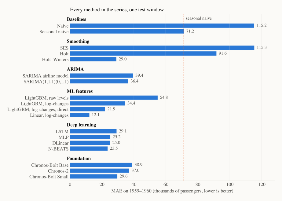
Links to each part: baselines · smoothing · ARIMA · ML features · deep learning · foundation models.
Taken at face value, the winner is clear: a plain linear regression on lagged log-changes (MAE 12.1), less than half the error of anything else. Before crowning it, remember the warning from Part 0: one test window is one exam. Let's give everyone a few more exams.
2. The re-match: rolling-origin evaluation#
In Part 0 we met rolling-origin evaluation: train on everything up to some point, forecast the next stretch, slide the cut-off forward, and repeat. Here we use six cut-offs, at the end of 1954, 1955, …, 1959. Each time, every method is re-fitted from scratch and forecasts the next 12 months. That gives six exams instead of one.
We re-ran the five methods that are cheap to refit: seasonal naive, Holt–Winters, the SARIMA airline model, LightGBM (direct, on log-changes) and the linear model on log-changes. The code is identical to the earlier parts; on the original split it reproduces their numbers exactly.
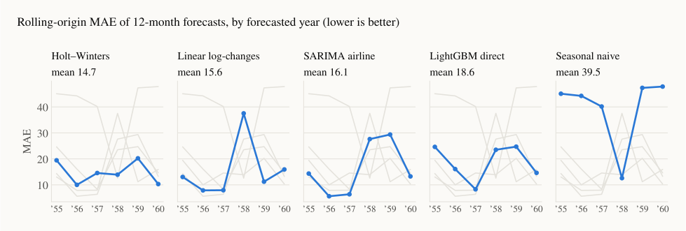
| Method | '55 | '56 | '57 | '58 | '59 | '60 | Mean |
|---|---|---|---|---|---|---|---|
| Holt–Winters | 19.5 | 10.0 | 14.6 | 13.9 | 20.2 | 10.3 | 14.7 |
| Linear, log-changes | 13.0 | 7.9 | 7.9 | 37.5 | 11.2 | 15.9 | 15.6 |
| SARIMA airline | 14.3 | 5.6 | 6.4 | 27.6 | 29.4 | 13.3 | 16.1 |
| LightGBM, direct | 24.6 | 16.1 | 8.3 | 23.5 | 24.7 | 14.6 | 18.6 |
| Seasonal naive | 45.1 | 44.2 | 40.2 | 12.6 | 47.3 | 47.8 | 39.5 |
The ranking changes:
- The "clear winner" isn't one. The linear model is excellent in most years but falls apart in 1958 (MAE 37.5), and its average lands in the middle of the pack.
- Holt–Winters wins on average without winning many individual years. Its worst year (20.2) is better than every other method's worst year. When you can only deploy one model and can't babysit it, being consistently decent is worth a lot.
- In 1958 the dumbest method wins. Air travel grew only 3.4% that year, during the 1957–58 recession, against the usual 12–19%. So "same as last year" was almost right. Every model that had learned "growth continues" overshot. No method from any era foresees a shock it has never seen.
- The top three are within 1.4 MAE of each other. Six exams aren't enough to separate them confidently. The real conclusion is "these three are all good here," not "X is best."
Notice what just happened: by changing only the evaluation, not the models, the story moved from "linear regression crushes everything" to "three methods tie, one is steadier." This is the most common way forecasting comparisons mislead, in blog posts and in papers alike.
3. Five lessons from the whole series#
1. Representation beats architecture. The biggest single jumps in the series didn't come from a cleverer model. They came from a better way of looking at the data:
| Same model | Raw levels | Log / log-changes |
|---|---|---|
| SARIMA airline model | 66.4 | 39.4 |
| LightGBM (recursive) | 54.8 | 34.4 |
Holt–Winters gets the same benefit through its multiplicative seasonality, and the deep-learning models through per-window normalisation. If a series grows by percentages, model it in percentages.
2. One test window lies; use several. Section 2 is the proof. With a single window you are partly measuring luck.
3. Always run the baselines. Seasonal naive costs one line of code. On the single test window, three later methods (naive, SES and Holt) failed to beat it. In the 1958 exam it beat everybody.
4. Complexity must pay rent. On one short, clean series, a three-parameter model from 1960 matches neural networks and 200-million-parameter foundation models. The newer methods earn their keep in settings this series doesn't have: many related series, outside information, long histories, multiple seasonal cycles.
5. A forecast without uncertainty is half a forecast. The SARIMA intervals in Part 2b covered all 24 test months. Chronos's 80% bands in Part 5 covered between 62% and 79%. Decisions (how much stock, how many staff) depend on the range, not just the middle line.
4. Which method should I use?#
A practical starting point. Each row says what to try first, not what to use forever:
| Your situation | Start with | Why |
|---|---|---|
| Any situation at all | Seasonal naive + rolling-origin evaluation | The bar to beat, and an honest way to measure |
| One or a few series, monthly or quarterly, regular patterns | ETS / Holt–Winters, then SARIMA | Fast, explainable, hard to beat on short series, with statistical prediction intervals |
| Hundreds to millions of related series (products, stores, sensors), with prices, promotions or holidays | One global LightGBM on lag, rolling and calendar features | Learns across series, uses outside information, won the M5 competition |
| Long histories, many series, several seasonal cycles, compute to spare | DLinear first, then N-BEATS / PatchTST-style networks | Learn features automatically, but check the linear model doesn't already match them |
| Little history, no time to model, or a quick strong baseline for many series | A foundation model zero-shot (e.g. Chronos-Bolt) | Good forecasts with no training; validate on your own data, since public benchmarks may have leaked into pretraining |
And three rules that hold in every row:
- Split by time, never at random.
- Transform first: logs for growth, differences for trends.
- Compare on several windows before you believe a ranking.
5. In code: a rolling-origin loop#
The re-match takes only a few lines. Here is the Holt–Winters vs seasonal naive part:
import numpy as np
import statsmodels.api as sm
from statsmodels.tsa.holtwinters import ExponentialSmoothing

y = sm.datasets.get_rdataset("AirPassengers").data["value"].to_numpy(dtype=float)

hw_err, sn_err = [], []
for end in range(72, 144, 12):              # train ends Dec 1954, Dec 1955, ..., Dec 1959
    train, test = y[:end], y[end:end + 12]
    hw = ExponentialSmoothing(train, trend="add", seasonal="mul", seasonal_periods=12,
                              initialization_method="estimated").fit()
    hw_err.append(np.mean(np.abs(test - hw.forecast(12))))
    sn_err.append(np.mean(np.abs(test - train[-12:])))   # seasonal naive

print(f"Holt-Winters mean MAE={np.mean(hw_err):.1f}  seasonal naive mean MAE={np.mean(sn_err):.1f}")
6. What this series didn't cover#
Forecasting is a big field. Natural next topics, if you want to keep going:
- Hierarchical forecasting: making store-level, region-level and national forecasts add up.
- Intermittent demand: series that are mostly zeros (spare parts), where MAPE breaks and Croston-type methods help.
- Multivariate models: several series that drive each other (VAR, multivariate deep models).
- Better uncertainty: conformal prediction, which wraps any model in intervals that are calibrated by construction. The series Conformal Prediction, Step by Step covers it, including adaptive intervals for this same dataset in Part 5.
- Anomaly detection and nowcasting: using the same tools to spot the unusual or estimate the present.
Recap#
- On one test window, a linear model on log-changes looked unbeatable. On six windows, Holt–Winters, that linear model and SARIMA tie, and Holt–Winters is the steadiest.
- The largest gains in the series came from transformations and honest evaluation, not from newer architectures.
- Newer eras don't replace older ones; they open new settings: many series, outside information, zero-shot forecasting.
- Start every project with seasonal naive, a time-based split and rolling-origin evaluation, then add complexity only when it pays.
Thanks for following Time Series, Era by Era. If you only remember one sentence from the series, make it this one: look at your data, beat the baseline, and test on more than one window.